My Autographed Laptop

Back in my university days the computer science club used to occasionally invite high profile speakers. I had a fairly old laptop at the time and I made a habit of taking it with me for autographs, to the total bewilderment of the speakers.

Since then, my laptop has followed me to conferences and has taken a few trips via snail mail. Here is the story of some of the more notable names that adorn its plastic shell.

RMS

The laptop was first blessed by Saint IGNUcius, of the church of Emacs, founder of the GNU project. You can see it on the right hand side of the keyboard below. The signatures near the keyboard tend to be a bit faded, as I was still using the laptop at the time.

RMS’ blessing was not without the requisite penance. I had an aluminum Tux sticker pasted on the back of the laptop and RMS took quick notice.

He promptly corrected the error by covering it with a GNU & Linux sticker. I have since committed the further sin of relocating the sticker to the location of the former Windows license and the penance of being a habitual vi user.

Bjarne Stroustrup

My next autograph came from Mr Stroustrup, who designed and implemented C++. You can see it on the left in this shot.

Stroustrup was confused as to why I would want his autograph. I explained that I was a C++/OpenGL demo scener in high school and that I was trying to get the autographs of my heroes on my laptop. His response was “that’s a neat little project you’ve started”.

Rasmus Leardorf

Next up is the co-author of PHP. Coincidentally, we attended the same undergraduate course. Rasmus’ talk was the first time I was introduced to the idea of using Valgrind to performance tune an interpreted language.

Don Knuth

Professor Knuth’s autograph was something I had coveted for some time. I was unlikely that I would be fortunate enough to attend one of his talks. So instead, I took a chance and sent him this letter:

After an exchange of snail mail, I had his autograph:

Guido van Rossum

Guido is the author and former BDFL of Python. I met Guido at PyCon several years ago without my laptop. I was originally planning on snail mailing him the machine, as I had with Knuth, but two years later I ran into him again at another PyCon.

I made a point of wearing the shirt below and was rewarded with a silly walk for my trouble.

Why

It blows my mind that we live in an era where the engineers who pioneered the first TTL logic circuit boards (which I believe is the Saturn V LVDC, but I could be wrong) are alive when everyone carries around a microprocessor in their pockets.

The rate of technological change is fast, and software is both the fastest and slowest thing that can be changed. That means that I can meet the Newtons and Maxwells of computer science today; they were my heroes growing up 🙂

Whos Next?

You’ll notice that there are a number of autographs that I haven’t described, mostly because they’re not public figures. My general rule is that anyone who has played a major part in writing a complex piece of software, or software in general, is welcome on the laptop.

I’m sad to have missed the opportunity to get the autographs of John McCarthy, Edsger Dijkstra and Dennis Ritchie. That being said, my current shortlist is:

• Ken Thompson
• Douglas McIlroy
• Linus Torvalds

If you know any of the people above, or can recommend anyone else, feel free to let them know I’m looking for an autograph 🙂

SQL: Nested Window Functions and Time Series

In an effort to keep up my grueling regime of publishing at least one blog post per year, I’ve decided to write today about a neat little problem I ran across. The problem is; how do you calculate the cumulative sum of a time series if there are transactions that reset the count to 0?

Naturally, there are ways to engineer around this problem without complex queries doing the heavy lifting (recording the current balance along side your transaction history, for example). However, if you occasionally find yourself being asked for a number crunch, half with the expectation of your response being:

…it’s not a bad idea to keep this query in your back pocket.

A Convoluted Example

Alice decides to start a bank. Her engineers are clever and they decide that they can save space in their transaction log by just reporting changes in the balance. They keep the current balance in another table and decide if Grace the auditor comes around, they’ll just sum up all of the transactions in their log. Good job guys.

Bob is an exceptional client with good credit history. Grace takes a quick glance at his balance history and decides everything looks fine. As she leafs through the other records and pauses at Sybil’s balance history. It’s massive. The problem is that Sybil’s been through a number of bankruptcies that should have set her balance to 0. She breaks the news to Alice. You can imagine that Alice was not too happy.

To fix the problem, the engineers decide to introduce a new transaction that resets the balance to 0.

The Data Set

In order to satisfy Grace, we’ve got to come up with a balance history for both Bob and Sybil using just transactions. Here’s our data set in Postgres SQL. We’ll use text and integer columns along with small numbers to simplify the problem.

CREATE TABLE transactions (
  id integer
  ,account text
  ,type text
  ,amount integer
);

INSERT INTO transactions
VALUES
  (1, 'bob', 'deposit', 5)
  ,(2, 'bob', 'withdrawal', -2)
  ,(3, 'bob', 'deposit', 3)
  ,(4, 'sybil', 'deposit', 5)
  ,(5, 'sybil', 'withdrawal', -2)
  ,(6, 'sybil', 'bankrupt', 0)
  ,(7, 'sybil', 'deposit' , 3)
  ,(8, 'sybil', 'deposit', 7)
  ,(9, 'sybil', 'bankrupt', 0)
  ,(10, 'sybil', 'deposit' , 5)
;

Simple Cumulative Sums

Our first job is to calculate Bob’s balance history. This section is a review of basic window functions. If you’re used to using them to create cumulative sums, feel free to skip ahead. Here’s what we’re trying to produce:

 id | account |    type    | amount | sum
----+---------+------------+--------+-----
  1 | bob     | deposit    |      5 |   5
  2 | bob     | withdrawal |     -2 |   3
  3 | bob     | deposit    |      3 |   6

A window function has two parts; the partition and the order. The partition defines which columns are going to be grouped together in the window. The order defines how to sort the rows in the window.

In the example above, we want to group transactions by their account. We then want to order them by their ID. Now, when we use the Sum function, it will sum from the first transaction in the partition, to the current row:

SELECT
  id
  ,account
  ,type
  ,amount
  ,sum(amount) OVER account
FROM transactions
WHERE account = 'bob'
WINDOW account AS (
  PARTITION BY account
  ORDER BY id
);

However, if we use the same query for Sybil, we run into our next problem.

 id | account |    type    | amount | sum
----+---------+------------+--------+-----
  4 | sybil   | deposit    |      5 |   5
  5 | sybil   | withdrawal |     -2 |   3
  6 | sybil   | bankrupt   |      0 |   3
  7 | sybil   | deposit    |      3 |   6
  8 | sybil   | deposit    |      7 |  13
  9 | sybil   | bankrupt   |      0 |  13
 10 | sybil   | deposit    |      5 |  18

Cumulative Sums With Resets

The trick to calculating Sybil’s balance is using a nested set of window functions to make the query sensitive to the transaction type. Here’s what we’re trying to achieve:

 id | account |    type    | amount | sum
----+---------+------------+--------+-----
  4 | sybil   | deposit    |      5 |   5
  5 | sybil   | withdrawal |     -2 |   3
  6 | sybil   | bankrupt   |      0 |   0
  7 | sybil   | deposit    |      3 |   3
  8 | sybil   | deposit    |      7 |  10
  9 | sybil   | bankrupt   |      0 |   0
 10 | sybil   | deposit    |      5 |   5

One possible solution is to try and subtract the cumulative sum using a CASE statement:

SELECT
  id
  ,account
  ,type
  ,amount
  ,CASE
    WHEN type = 'bankrupt' THEN
      -1*sum(amount) OVER account
    ELSE
      sum(amount) OVER account
  END AS sum
FROM transactions
WHERE account = 'sybil'
WINDOW account AS (
  PARTITION BY account
  ORDER BY id
);

The trouble with this approach is that the window function does not use the output of the last row to calculate the next row. The only thing we’ve done is to alter the values of the bankrupt transactions:

 id | account |    type    | amount | sum
----+---------+------------+--------+-----
  4 | sybil   | deposit    |      5 |   5
  5 | sybil   | withdrawal |     -2 |   3
  6 | sybil   | bankrupt   |      0 |  -3
  7 | sybil   | deposit    |      3 |   6
  8 | sybil   | deposit    |      7 |  13
  9 | sybil   | bankrupt   |      0 | -13
 10 | sybil   | deposit    |      5 |  18

Nesting window functions solves this problem. We’ll build up the query by first identifying the transactions that reset the count:

SELECT
  id
  ,account
  ,type
  ,amount
  ,(type = 'bankrupt')::int AS do_reset
FROM transactions
WHERE account = 'sybil'
;

Running that query we get:

 id | account |    type    | amount | do_reset
----+---------+------------+--------+----------
  4 | sybil   | deposit    |      5 |        0
  5 | sybil   | withdrawal |     -2 |        0
  6 | sybil   | bankrupt   |      0 |        1
  7 | sybil   | deposit    |      3 |        0
  8 | sybil   | deposit    |      7 |        0
  9 | sybil   | bankrupt   |      0 |        1
 10 | sybil   | deposit    |      5 |        0

Casting boolean values to integers allows us to then perform a cumulative sum over do_reset. This sum will allow us to group transactions chronologically, by their association to a resetting transaction.

SELECT
  id
  ,account
  ,type
  ,amount
  ,sum((type = 'bankrupt')::int) OVER account AS reset_id
FROM transactions
WHERE account = 'sybil'
WINDOW account AS (
  PARTITION BY account
  ORDER BY id
);

Running that query we get:

 id | account |    type    | amount | reset_id
----+---------+------------+--------+----------
  4 | sybil   | deposit    |      5 |        0
  5 | sybil   | withdrawal |     -2 |        0
  6 | sybil   | bankrupt   |      0 |        1
  7 | sybil   | deposit    |      3 |        1
  8 | sybil   | deposit    |      7 |        1
  9 | sybil   | bankrupt   |      0 |        2
 10 | sybil   | deposit    |      5 |        2

Finally, we can nest this query inside another window function, and perform a cumulative sum on amount, using the reset_id we’ve just created:

SELECT
  id
  ,account
  ,type
  ,amount
  ,sum(amount) OVER resets
FROM (
  SELECT
    id
    ,account
    ,type
    ,amount
    ,sum((type = 'bankrupt')::int) OVER account AS reset_id
  FROM transactions
  WINDOW account AS (
    PARTITION BY account
    ORDER BY id
  )
) t
WINDOW resets AS (
  PARTITION BY
    account
    ,reset_id
  ORDER BY id
);

Running the query we get the values we expect for both Bob and Sybil. Huzzah!

 id | account |    type    | amount | sum
----+---------+------------+--------+-----
  1 | bob     | deposit    |      5 |   5
  2 | bob     | withdrawal |     -2 |   3
  3 | bob     | deposit    |      3 |   6
  4 | sybil   | deposit    |      5 |   5
  5 | sybil   | withdrawal |     -2 |   3
  6 | sybil   | bankrupt   |      0 |   0
  7 | sybil   | deposit    |      3 |   3
  8 | sybil   | deposit    |      7 |  10
  9 | sybil   | bankrupt   |      0 |   0
 10 | sybil   | deposit    |      5 |   5

Conclusion

Window functions are a really good solution to processing time series with chronologically related data. This post scratches the surface of what’s possible.

So, the next time your boss asks you to process some time series data, consider giving window functions a try.

range(n): A Deceptively Complex Program

I’ve been itching to write this article since I authored Python vs Copy on Write last year. To recap, I found myself awake at 4 AM trying to performance tune the cache on a long running ETL written in Python.

In a flash of pizza fueled, sleep deprived clarity, I remembered Brandon Rhodes’ talk on Python, Linkers, and Virtual Memory; because of reference counting, Python cannot take advantage of the Copy on Write optimization provided by the OS. An hour later I had a patch ready for our staging environment.

If you read my previous article, you may have been under the impression that my fix was a silver bullet and you’d be partially right.

The patch did have the intended effect of reducing the runtime of the areas of code that used the cache, but to my horror I found that I had created another bottleneck. We use psycopg2 to query our database, and our code was now spending hours running this line to create the new cache:

cursor.fetchall()

Thinking back to my long night of coding, I remember noticing that for some reason the range(very large number) function that I was using to generate the dummy cache in my experiments was taking a long time to run. So, I hypothesized that allocating a large list to store the fetchall results was bottle necking my process.

I refactored, reran the ETL in our staging environment and waited as fast as I could. Like magic, the ETL finished with more than a 40% reduction in runtime and I could console myself in that my sleep schedule would return to normal.

But, there was always the lingering question as to why large list allocations take so much time. So grab your gear, prime your Python, C and Unix cheat sheets and get ready for a deep dive into the python interpreter.

Tools

To avoid reading through the C Python interpreter’s source, we’ll run a number of Unix profiling tools on Ubuntu 16.04 against some simple examples. We will start with ltrace for standard library traces and strace for system call traces.

Then we will move onto Valgrind to thoroughly diagnose the problem. Valgrind is a framework that contains a number of dynamic analysis tools. Its Memcheck tool is commonly used to detect memory leaks. For our problem we will be using Massif, DHAT and Callgrind from the Valgrind suite.

We will start with Massif for heap profiling. Massif provides a timeline of allocated memory. We will then use DHAT for some summarized allocation statistics.

The bulk of our work will focus on Callgrind to profile the call history using a call graph. KCachegrind will let us visualize the call graph and determine exactly where our cycles are being spent.

I should note that part of my purpose in writing this blog is to demonstrate the use of these tools. Were I to perform a task like this for practical purposes, I would probably reach for Memcheck and Callgrind, and likely skip the rest.

Feel free to follow along by checking out this git repository. In most cases, I’ve encapsulated examples into single bash scripts. In this article, I’ll make a note of the path of the example I’m using and cat the bash script so that you can see its contents. I’ve also produced a docker image that will provide a version of Python 2.7 compiled to be run with Valgrind. In order to install docker, run the following:

$ sudo apt-get install docker.io
$ sudo adduser $USER docker

You may have to log out and log back in, in order to be recognized as a member of the docker group.

The Benchmark

To start, let’s go back to the program that started this whole investigation:

src/python/benchmark.py

#!/usr/bin/env python
# -*- coding: utf-8 -*-

range(10000000)

Remember the original hypothesis; allocating large lists of integers caused an increase in runtime. The range function in this case is a very easy way to create a large list of integers. The size parameter passed to range is somewhat arbitrary. It has to be sufficiently large to be noticeable on the machine you’re running on. In my case, the magic number is 10,000,000.

A brief note on the differences between Python 2.7 and Python 3; range is implemented differently. We can measure the difference using the Unix time command:

src/python/$ time python2.7 benchmark.py

real 0m0.404s
user 0m0.220s
sys 0m0.180s

‘real’ is the time from start to finish. ‘user’ is the time spent in user-mode code, outside of the kernel. ‘sys’ is the time spent in the kernel via system calls. Compare this runtime to the results from Python 3:

src/python/$ time python3.5 benchmark.py

real 0m0.040s
user 0m0.032s
sys 0m0.004s

Instead of allocating a populated list, Python 3 creates a Range object. I haven’t verified, but I assume the range object operates like a generator. To eliminate this complexity, we’ll stick with Python 2.7.

The C Python interpreter is a complex piece of software. In order to establish a baseline for understanding its operation, we’ll create a naively comparable program in C:

src/c/benchmark.c

#include <stdlib.h>

#define LENGTH 10000000

int main() {
  // Allocate the memory.
  int * buffer = malloc(LENGTH * sizeof(int));

  // Seed the memory.
  for (int index = 0; index < LENGTH; index++) {
    buffer[index] = index;
  }

  // Free the memory.
  free (buffer);

  return 0;
}

Note that you will need to install some software to get this program to compile:

$ sudo apt-get install build-essential

A quick check with the time command:

src/c/$ make
rm -f benchmark
rm -f *.out.*
gcc -g -o benchmark benchmark.c

src/c/$ time ./benchmark

real 0m0.072s
user 0m0.064s
sys 0m0.004s

I understand that this is an apples to oranges comparison, but the differences we find should be illuminating. The simplified C program will also let us explore our tool set with something that is easy to understand. Right, it’s time to learn how to defend your runtime against a blogger armed with apple and an orange.

ltrace

ltrace is a program that lets us take a peek at the standard library calls being made by a program. As our C and Python programs are somewhat simple, ltrace should give us a quick idea of how different these programs are. First, the C program:

src/c/ltrace

src/c/$ cat ltrace
#!/bin/sh
ltrace ./benchmark

src/c/$ ./ltrace
__libc_start_main(0x400566, 1, 0x7ffdc5a20818, 0x400590 <unfinished ...>
malloc(40000000) = 0x7fa98820b010
free(0x7fa98820b010) = <void>
+++ exited (status 0) +++

As expected, the C program allocated all of the 40 MB of memory with a single command (malloc).

Second, the Python program. Running ltrace directly on the python script is somewhat unwieldy. We’ll have to filter the results. Lets start with a summary of the calls:

src/python/ltrace

% time     seconds  usecs/call     calls      function
------ ----------- ----------- --------- --------------------
 47.46   10.684727          43    246094 free
 44.10    9.927329          40    245504 malloc
  2.60    0.585793          39     14734 memcpy
  1.55    0.348615          40      8530 memset
  1.26    0.283193          40      6962 strlen
  1.03    0.231403          39      5819 memcmp
  0.52    0.116267          43      2688 strcmp
  0.41    0.091900          40      2248 __ctype_b_loc
  0.18    0.041460          39      1040 realloc
  0.18    0.040438       13479         3 qsort
  0.11    0.023975          39       602 strchr

...

It seems that our script is spending the majority of its time on memory operations. Digging deeper into the mallocs, this script sorts and counts the calls based on the buffer size.

src/python/malloc

src/python/$ cat malloc
#!/bin/sh
ltrace -e malloc -l python python benchmark.py 2>&1 | sed "s/).*//" | sed "s/.*(//" | sort -nr | uniq -c

$ ./malloc
1 80000000
1 36654
4 36032
1 25593
1 25474
1 20808
1 19945
1 19712

...

     1 1141
     1 1105
     1 1053
     1 1034
243929 992
     1 991
     1 990
     1 978
     1 977

...

Two interesting observations can be made. The first is that there is a very large allocation being made; double the size of the C allocation. As we are interested in runtime, we also find that python is performing 243929 allocations of 992 byte buffers, or 242 MB.

As an aside, if you’d like to play around with ltrace and python, you can set the range in the benchmark program to something a bit more manageable, like 100. The output is still fairly unwieldy:

src/python/$ ltrace python -c "range(100)"
__libc_start_main(0x49dab0, 2, 0x7ffed23f7ab8, 0x5d71b0 <unfinished ...>
getenv("PYTHONHASHSEED")                         = nil
getenv("PYTHONINSPECT")                          = nil
getenv("PYTHONUNBUFFERED")                       = nil
getenv("PYTHONNOUSERSITE")                       = nil
getenv("PYTHONWARNINGS")                         = nil
fileno(0x7f26b16ec8e0)                           = 0

...

Among other things, we can see some of the built in functions being copied around in memory:

...

strlen("print")                                  = 5
memcpy(0x7f1bf84e56b4, "print\0", 6)             = 0x7f1bf84e56b4
strlen("range")                                  = 5
memcpy(0x7f1bf84e56e4, "range\0", 6)             = 0x7f1bf84e56e4
strlen("raw_input")                              = 9
memcpy(0x7f1bf84e5714, "raw_input\0", 10)        = 0x7f1bf84e5714

...

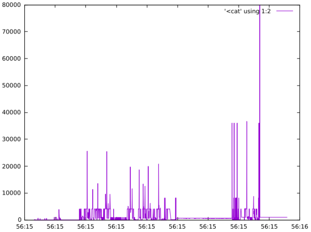
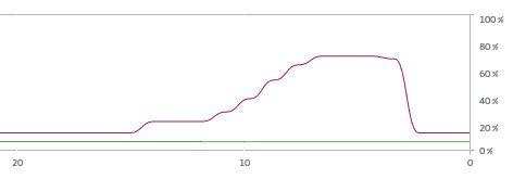
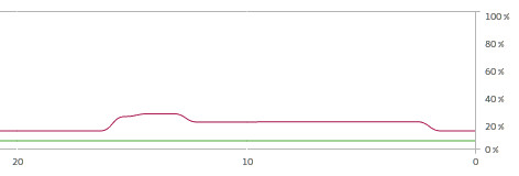
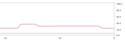
We can also combine ltrace with tools like gnuplot to visually see the malloc calls over time. Note the size of the range parameter has been reduced so that we can see other allocations performed by the interpreter:

src/python/timeline

src/python/$ cat timeline
#!/bin/sh
ltrace -tt -e malloc -l python python -c "range(10000)" 2>&1 | grep "malloc" | sed "s/python.*(//" | sed "s/).*//" | gnuplot -p -e "set xdata time; set timefmt '%H:%M:%S'; plot '<cat' using 1:2 with lines"

strace

Since we’re talking about ltrace, we may as well cover strace. strace lets us take a look at the system calls our programs are making. System calls are like functions that request the services from the kernel. They typically deal with resource allocation requests.

You can find a categorized list of them at System Calls for Developers. System calls are typically not made directly in code. Instead, wrapper functions in the form of a standard library are used. strace intecrepts these calls and prints them for inspection.

As before, we will start with our C program. We will filter everything except memory related calls:

src/c/strace

src/c/$ cat strace
#!/bin/sh
strace -e memory ./benchmark

src/c/$ ./strace
brk(NULL) = 0xaf0000
mmap(NULL, 8192, PROT_READ|PROT_WRITE, MAP_PRIVATE|MAP_ANONYMOUS, -1, 0) = 0x7f5e8b790000
mmap(NULL, 125519, PROT_READ, MAP_PRIVATE, 3, 0) = 0x7f5e8b771000
mmap(NULL, 3967392, PROT_READ|PROT_EXEC, MAP_PRIVATE|MAP_DENYWRITE, 3, 0) = 0x7f5e8b1a4000
mprotect(0x7f5e8b363000, 2097152, PROT_NONE) = 0
mmap(0x7f5e8b563000, 24576, PROT_READ|PROT_WRITE, MAP_PRIVATE|MAP_FIXED|MAP_DENYWRITE, 3, 0x1bf000) = 0x7f5e8b563000
mmap(0x7f5e8b569000, 14752, PROT_READ|PROT_WRITE, MAP_PRIVATE|MAP_FIXED|MAP_ANONYMOUS, -1, 0) = 0x7f5e8b569000
mmap(NULL, 4096, PROT_READ|PROT_WRITE, MAP_PRIVATE|MAP_ANONYMOUS, -1, 0) = 0x7f5e8b770000
mmap(NULL, 4096, PROT_READ|PROT_WRITE, MAP_PRIVATE|MAP_ANONYMOUS, -1, 0) = 0x7f5e8b76f000
mmap(NULL, 4096, PROT_READ|PROT_WRITE, MAP_PRIVATE|MAP_ANONYMOUS, -1, 0) = 0x7f5e8b76e000
mprotect(0x7f5e8b563000, 16384, PROT_READ) = 0
mprotect(0x600000, 4096, PROT_READ) = 0
mprotect(0x7f5e8b792000, 4096, PROT_READ) = 0
munmap(0x7f5e8b771000, 125519) = 0
mmap(NULL, 40001536, PROT_READ|PROT_WRITE, MAP_PRIVATE|MAP_ANONYMOUS, -1, 0) = 0x7f5e88b7e000
munmap(0x7f5e88b7e000, 40001536) = 0
+++ exited with 0 +++

The two calls of interest are the last two prior to exit (mmap and munmap), which correspond to the malloc and free calls respectively. We can infer this correspondence because mmap and munmap are called with a size of 40,001,536.

On to the python program. We’ll summarize the results again with the -c flag to reduce the size of the output:

src/python/strace

src/python/$ cat strace
#!/bin/sh
strace -c -e memory python benchmark.py

src/python/$ ./strace
% time     seconds  usecs/call     calls    errors syscall
------ ----------- ----------- --------- --------- ----------------
100.00    0.000264           0     61837           brk
  0.00    0.000000           0        29           mmap
  0.00    0.000000           0        14           mprotect
  0.00    0.000000           0         2           munmap
------ ----------- ----------- --------- --------- ----------------
100.00    0.000264                 61882           total

It seems the bulk of our memory related system calls are brk calls and not mmap calls. What’s the difference between brk and mmap? brk is typically used for small allocations. mmap on the other hand lets you allocate independent regions without being limited to a single chunk of memory. It useful for avoiding issues like memory fragmentation when allocating large memory blocks.

As we found with ltrace, it seems that in addition to the large block of memory allocated by mmap, the python process also allocates a large number of small memory blocks with brk.

The Environment

So far, ltrace and strace have been useful for getting an overall understanding of the differences between the C and Python programs. However, the results we’ve gotten have been either too detailed or too summarized to draw useful conclusions. We need to try something completely different.

To dig deeper into this problem, we’ll need better tooling. That’s where Valgrind comes in. Valgrind is a framework that contains a number of dynamic analysis tools. There’s a catch; we will need to compile our programs for debugging.

For the C program, this process is easy; it’s already compiled this way via its Makefile. All you need to start running Valgrind is to install valgrind and KCachegrind:

$ sudo apt-get install valgrind kcachegrind

Compiling Python for use with Valgrind is a bit more involved. There’s a README and a detailed stack overflow post on the subject. Fortunately, your trusty narrator has produced a docker image. Spinning up an instance of Python that you can Valgrind is as easy as:

src/python/valgrind

src/python/$ cat valgrind
#!/bin/sh
docker run -it -v ${PWD}/results:/results rishiramraj/range_n bash

src/python/$ ./valgrind
root@3d0bd3df72f0:/tmp/python2.7-2.7.12# ./python -c 'print("hello world")'
hello world
[21668 refs]
root@3d0bd3df72f0:/tmp/python2.7-2.7.12#

If you’d like to understand the process of compiling Python for use with Valgrind, take a look at env/Dockerfile in the github repo.

Massif

The first Valgrind tool we’ll bring to bear is called Massif. Massif will take periodic snapshots of our program’s heap and stack. It should give us a better idea of how Python is allocating memory over time.

By default, Massif does not track stack memory as stack profiling is slow. We have the luxury of tracing stack as our programs are fairly short running. Another consideration when using Massif is the time unit. Massif can measure time along three different dimensions; instructions executed (i), milliseconds (ms) and bytes allocated (B). The choice of dimension will depend on what you want to highlight. For short programs, bytes allocated often produces the most useful timelines, but feel free to experiment.

Lets start by running the C program with bytes allocated as the time parameter. We should expect a single large peak in the timeline.

src/c/massif

src/c/$ cat massif
#!/bin/sh
valgrind --tool=massif --stacks=yes --time-unit=B ./benchmark

src/c/$ ./massif
==5650== Massif, a heap profiler
==5650== Copyright (C) 2003-2015, and GNU GPL'd, by Nicholas Nethercote
==5650== Using Valgrind-3.11.0 and LibVEX; rerun with -h for copyright info
==5650== Command: ./benchmark
==5650==
==5650==

$ ms_print massif.out.10310
--------------------------------------------------------------------------------
Command:            ./benchmark
Massif arguments:   --stacks=yes --time-unit=B
ms_print arguments: massif.out.10310
--------------------------------------------------------------------------------

    MB
38.15^                                    #
     |                                    #::::::::::::::::::::::::::::::::::
     |                                    #
     |                                    #
     |                                    #
     |                                    #
     |                                    #
     |                                    #
     |                                    #
     |                                    #
     |                                    #
     |                                    #
     |                                    #
     |                                    #
     |                                    #
     |                                    #
     |                                    #
     |                                    #
     |                                    #
     |                                    #
   0 +----------------------------------------------------------------------->MB
     0                                                                   76.51

Number of snapshots: 60
 Detailed snapshots: [4, 5, 6, 9, 14, 31, 38, 42, 51 (peak)]

--------------------------------------------------------------------------------
  n        time(B)         total(B)   useful-heap(B) extra-heap(B)    stacks(B)
--------------------------------------------------------------------------------
  0              0                0                0             0            0
  1          3,952              624                0             0          624
  2          7,304            2,456                0             0        2,456

...

 51     40,201,032       40,001,800       40,000,000         1,480          320
100.00% (40,000,000B) (heap allocation functions) malloc/new/new[], --alloc-fns, etc.
->100.00% (40,000,000B) 0x400576: main (benchmark.c:7)

...

The output contains a number of parts: the timeline, a summary of the snapshots, normal snapshots and detailed snapshots. The timeline uses different characters for the various types of snapshots. “:” is used for normal snapshots. “@” is used for detailed snapshots. The peak is illustrated with “#”. The snapshot summary follows the timeline indicating which snapshots are detailed and where the peak occurs.

Normal snapshots present the following information:

• n: The snapshot number.
• time(B): The time it was taken.
• total(B): The total memory consumption at that point.
• useful-heap(B): The number of useful heap bytes allocated.
• extra-heap(B): Bytes in excess of what the program asked for.
• stacks(B): The size of the stack.

Detailed snapshots also provide an allocation tree, which shows locations within the code and their associated percentage of memory usage. As most allocations use either new or malloc, these calls often end up at the top of the tree, accounting for 100% of the memory usage. In our example above, the peak snapshot (snapshot 51) occurs when malloc is called from main, and accounts for 100% of the memory usage.

Now on to the Python program. Unfortunately, the docker volume writes files as root, so the file permissions will have to be changed before you can run ms_print.

src/python/massif

src/python/$ cat massif
#!/bin/sh
docker run -it -v ${PWD}/results:/results rishiramraj/range_n valgrind --tool=massif --stacks=yes --massif-out-file=/results/massif.out --time-unit=B ./python -c 'range(10000000)'

src/python/$ ./massif
==1== Massif, a heap profiler
==1== Copyright (C) 2003-2015, and GNU GPL'd, by Nicholas Nethercote
==1== Using Valgrind-3.11.0 and LibVEX; rerun with -h for copyright info
==1== Command: ./python -c range(10000000)
==1==
[21668 refs]
==1==

src/python/$ cd results
src/python/results/$ sudo chown $USER:$USER massif.out
src/python/results/$ ms_print massif.out
--------------------------------------------------------------------------------
Command:            ./python -c range(10000000)
Massif arguments:   --stacks=yes --massif-out-file=/results/massif.out --time-unit=B
ms_print arguments: massif.out
--------------------------------------------------------------------------------

    MB
482.6^                                                        :   @
     |                                  @@#::::::@::::::::::::::::@:
     |                                 @@@#:: :::@: :::::: :::::::@:
     |                               @@@@@#:: :::@: :::::: :::::::@:
     |                            @@@@ @@@#:: :::@: :::::: :::::::@::
     |                           @@ @@ @@@#:: :::@: :::::: :::::::@:::
     |                         @@@@ @@ @@@#:: :::@: :::::: :::::::@:::
     |                      @@@@@@@ @@ @@@#:: :::@: :::::: :::::::@::::
     |                    @@@@ @@@@ @@ @@@#:: :::@: :::::: :::::::@::::
     |                  @@@@@@ @@@@ @@ @@@#:: :::@: :::::: :::::::@:::::
     |                @@@@@@@@ @@@@ @@ @@@#:: :::@: :::::: :::::::@::::::
     |              @@@@@@@@@@ @@@@ @@ @@@#:: :::@: :::::: :::::::@:::::@
     |             @@@@@@@@@@@ @@@@ @@ @@@#:: :::@: :::::: :::::::@:::::@:
     |          @@@@@@@@@@@@@@ @@@@ @@ @@@#:: :::@: :::::: :::::::@:::::@:
     |       :::@@ @@@@@@@@@@@ @@@@ @@ @@@#:: :::@: :::::: :::::::@:::::@::
     |       @::@@ @@@@@@@@@@@ @@@@ @@ @@@#:: :::@: :::::: :::::::@:::::@::
     |    :@@@::@@ @@@@@@@@@@@ @@@@ @@ @@@#:: :::@: :::::: :::::::@:::::@:::
     |  :::@ @::@@ @@@@@@@@@@@ @@@@ @@ @@@#:: :::@: :::::: :::::::@:::::@:::
     |  :::@ @::@@ @@@@@@@@@@@ @@@@ @@ @@@#:: :::@: :::::: :::::::@:::::@::::
     |  :::@ @::@@ @@@@@@@@@@@ @@@@ @@ @@@#:: :::@: :::::: :::::::@:::::@::::
   0 +----------------------------------------------------------------------->GB
     0                                                                   5.911

Number of snapshots: 79
 Detailed snapshots: [5, 6, 10, 11, 12, 13, 14, 15, 16, 17, 18, 19, 20, 21, 22, 23, 24, 25, 26, 27, 28, 29, 30, 31, 32, 33 (peak), 39, 58, 68, 78]

--------------------------------------------------------------------------------
  n        time(B)         total(B)   useful-heap(B) extra-heap(B)    stacks(B)
--------------------------------------------------------------------------------
  0              0                0                0             0            0
  1     86,521,128        1,987,800        1,848,921       121,615       17,264
  2    201,080,664       82,752,584       82,565,124       184,628        2,832
  3    297,978,512       96,346,400       95,945,124       398,708        2,568
  4    417,445,088      113,111,392      112,446,124       662,724        2,544
  5    489,564,720      123,233,088      122,408,124       822,116        2,848

...

 33  3,184,292,720      501,388,288      494,608,124     6,777,316        2,848
98.65% (494,608,124B) (heap allocation functions) malloc/new/new[], --alloc-fns, etc.
->98.64% (494,591,075B) 0x466C1C: PyObject_Malloc (obmalloc.c:986)
| ->98.64% (494,591,075B) 0x467676: _PyObject_DebugMallocApi (obmalloc.c:1494)
|   ->98.28% (492,756,684B) 0x467565: _PyMem_DebugMalloc (obmalloc.c:1444)
|   | ->82.18% (412,061,000B) 0x43F3D4: fill_free_list (intobject.c:52)
|   | | ->82.18% (412,050,000B) 0x43F4AD: PyInt_FromLong (intobject.c:104)
|   | | | ->82.18% (412,043,000B) 0x4CA61D: builtin_range (bltinmodule.c:2008)
|   | | | | ->82.18% (412,043,000B) 0x571B0F: PyCFunction_Call (methodobject.c:81)
|   | | | |   ->82.18% (412,043,000B) 0x4DE975: call_function (ceval.c:4350)
|   | | | |     ->82.18% (412,043,000B) 0x4D91F5: PyEval_EvalFrameEx (ceval.c:2987)
|   | | | |       ->82.18% (412,043,000B) 0x4DC0CB: PyEval_EvalCodeEx (ceval.c:3582)
|   | | | |         ->82.18% (412,043,000B) 0x4CE7AE: PyEval_EvalCode (ceval.c:669)
|   | | | |           ->82.18% (412,043,000B) 0x50FEF4: run_mod (pythonrun.c:1376)
|   | | | |             ->82.18% (412,043,000B) 0x50FDAD: PyRun_StringFlags (pythonrun.c:1339)
|   | | | |               ->82.18% (412,043,000B) 0x50E740: PyRun_SimpleStringFlags (pythonrun.c:974)
|   | | | |                 ->82.18% (412,043,000B) 0x415FE5: Py_Main (main.c:584)
|   | | | |                   ->82.18% (412,043,000B) 0x414CF4: main (python.c:20)
|   | | | |
|   | | | ->00.00% (7,000B) in 1+ places, all below ms_print's threshold (01.00%)
|   | | |
|   | | ->00.00% (11,000B) in 1+ places, all below ms_print's threshold (01.00%)
|   | |
|   | ->15.96% (80,002,024B) 0x4438E6: PyList_New (listobject.c:152)
|   | | ->15.96% (80,000,032B) 0x4CA5EF: builtin_range (bltinmodule.c:2004)
|   | | | ->15.96% (80,000,032B) 0x571B0F: PyCFunction_Call (methodobject.c:81)
|   | | |   ->15.96% (80,000,032B) 0x4DE975: call_function (ceval.c:4350)
|   | | |     ->15.96% (80,000,032B) 0x4D91F5: PyEval_EvalFrameEx (ceval.c:2987)
|   | | |       ->15.96% (80,000,032B) 0x4DC0CB: PyEval_EvalCodeEx (ceval.c:3582)
|   | | |         ->15.96% (80,000,032B) 0x4CE7AE: PyEval_EvalCode (ceval.c:669)
|   | | |           ->15.96% (80,000,032B) 0x50FEF4: run_mod (pythonrun.c:1376)
|   | | |             ->15.96% (80,000,032B) 0x50FDAD: PyRun_StringFlags (pythonrun.c:1339)
|   | | |               ->15.96% (80,000,032B) 0x50E740: PyRun_SimpleStringFlags (pythonrun.c:974)
|   | | |                 ->15.96% (80,000,032B) 0x415FE5: Py_Main (main.c:584)
|   | | |                   ->15.96% (80,000,032B) 0x414CF4: main (python.c:20)
|   | | |
|   | | ->00.00% (1,992B) in 1+ places, all below ms_print's threshold (01.00%)
|   | |
|   | ->00.14% (693,660B) in 1+ places, all below ms_print's threshold (01.00%)
|   |
|   ->00.37% (1,834,391B) in 1+ places, all below ms_print's threshold (01.00%)
|
->00.00% (17,049B) in 1+ places, all below ms_print's threshold (01.00%)

...

Two interesting observations can be drawn from this output that corroborate our findings with ltrace and strace. The first thing we observe is from the timeline; Python is allocating an order of magnitude more memory when compared to the C program (around 480 MB). This memory grows over time instead of being allocated all at once.

The second thing we observe is from the detailed snapshot of the peak; something other than the large list allocation made by PyList_New is consuming the bulk of the allocated memory. This function is called fill_free_list and likely accounts for the 243929 allocations we saw earlier.

This snapshot gives us a partial look into the internals the C Python interpreter. It’s interesting to note that PyList_New and fill_free_list have a common ancestor in builtin_range. If we were brave enough, we could dive into the source code at this point. Fortunately there’s better tooling we can use to save us a bit of time.

DHAT

Before we dive into the code using callgrind, let’s see if we can figure out how the additional memory we identified with Massif is being used. For that job we will use DHAT, which provides summarized statistics on heap allocations. Back to our C program:

src/c/dhat

src/c/$ cat dhat
#!/bin/sh
valgrind --tool=exp-dhat ./benchmark

src/c/$ ./dhat
==17163== DHAT, a dynamic heap analysis tool
==17163== NOTE: This is an Experimental-Class Valgrind Tool
==17163== Copyright (C) 2010-2015, and GNU GPL'd, by Mozilla Inc
==17163== Using Valgrind-3.11.0 and LibVEX; rerun with -h for copyright info
==17163== Command: ./benchmark
==17163==
==17163==
==17163== ======== SUMMARY STATISTICS ========
==17163==
==17163== guest_insns:  100,110,715
==17163==
==17163== max_live:     40,000,000 in 1 blocks
==17163==
==17163== tot_alloc:    40,000,000 in 1 blocks
==17163==
==17163== insns per allocated byte: 2
==17163==
==17163==
==17163== ======== ORDERED BY decreasing "max-bytes-live": top 10 allocators ========
==17163==
==17163== -------------------- 1 of 10 --------------------
==17163== max-live:    40,000,000 in 1 blocks
==17163== tot-alloc:   40,000,000 in 1 blocks (avg size 40000000.00)
==17163== deaths:      1, at avg age 100,001,087 (99.89% of prog lifetime)
==17163== acc-ratios:  0.00 rd, 1.00 wr  (0 b-read, 40,000,000 b-written)
==17163==    at 0x4C2BE7F: malloc (in /usr/lib/valgrind/vgpreload_exp-dhat-amd64-linux.so)
==17163==    by 0x400577: main (benchmark.c:7)

...

DHAT provides a number of summary statistics followed by a sorted list of memory allocators. Here are a number of definitions for terms used by the tool:

• block: A memory allocation; i.e. a call to malloc.
• guest_insns: Total number of instructions.
• max_live: The maximum number of blocks simultaneously allocated.
• tot_alloc: Memory allocation over the history of the program.
• deaths: Memory deallocation over the history of the program.
• acc-ratios: Read and write access ratios.

Understanding how to interpret the results from DHAT is the key to its usefulness. For example, an average death that is comparable to the length of the program implies that memory is all being deallocated at the end.

Read or write ratios of less than 1 imply that memory is either not being read from or written to. DHAT will also provide access counts per offset into a buffer, to make alignment problems easier to diagnose. An alignment problem will show up as a portion of the block that is not accessed and therefore filled with 0 counts. We’ll see a offset matrix in the Python example.

In our C example, we observe 100 million instructions which are likely used to seed the block. We also see a 40MB memory allocation as expected. By looking at the deaths measurement, the allocation lives for the duration of the programs execution. The allocation ratios tell us that the allocation is only written to once and never read. Now for the Python example:

src/python/dhat

src/python/$ cat dhat
#!/bin/sh
docker run -it rishiramraj/range_n valgrind --tool=exp-dhat ./python -c 'range(10000000)'

src/python/$ ./dhat
==1== DHAT, a dynamic heap analysis tool
==1== NOTE: This is an Experimental-Class Valgrind Tool
==1== Copyright (C) 2010-2015, and GNU GPL'd, by Mozilla Inc
==1== Using Valgrind-3.11.0 and LibVEX; rerun with -h for copyright info
==1== Command: ./python -c range(10000000)
==1==
[21668 refs]
==1==
==1== ======== SUMMARY STATISTICS ========
==1==
==1== guest_insns:  2,753,608,005
==1==
==1== max_live:     499,221,126 in 429,745 blocks
==1==
==1== tot_alloc:    501,946,111 in 439,591 blocks
==1==
==1== insns per allocated byte: 5
==1==
==1==
==1== ======== ORDERED BY decreasing "max-bytes-live": top 10 allocators ========
==1==
==1== -------------------- 1 of 10 --------------------
==1== max-live:    416,656,000 in 416,656 blocks
==1== tot-alloc:   416,656,000 in 416,656 blocks (avg size 1000.00)
==1== deaths:      416,656, at avg age 1,814,285,338 (65.88% of prog lifetime)
==1== acc-ratios:  2.91 rd, 4.46 wr  (1,216,634,728 b-read, 1,860,368,408 b-written)
==1==    at 0x4C2BE7F: malloc (in /usr/lib/valgrind/vgpreload_exp-dhat-amd64-linux.so)
==1==    by 0x466C1D: PyObject_Malloc (obmalloc.c:986)
==1==    by 0x467677: _PyObject_DebugMallocApi (obmalloc.c:1494)
==1==    by 0x467566: _PyMem_DebugMalloc (obmalloc.c:1444)
==1==    by 0x43F3D5: fill_free_list (intobject.c:52)
==1==    by 0x43F4AE: PyInt_FromLong (intobject.c:104)
==1==    by 0x4CA61E: builtin_range (bltinmodule.c:2008)
==1==    by 0x571B10: PyCFunction_Call (methodobject.c:81)
==1==    by 0x4DE976: call_function (ceval.c:4350)
==1==    by 0x4D91F6: PyEval_EvalFrameEx (ceval.c:2987)
==1==    by 0x4DC0CC: PyEval_EvalCodeEx (ceval.c:3582)
==1==    by 0x4CE7AF: PyEval_EvalCode (ceval.c:669)
==1==
==1== Aggregated access counts by offset:
==1==
==1== [   0]  1666624 1666624 1666624 1666624 1666624 1666624 1666624 1666624 1249968 1249968 1249968 1249968 1666624 1249968 1249968 1249968
==1== [  16]  1874953 1874953 1874953 1874953 1874953 1874953 1874953 1874953 3124916 3124916 3124916 3124916 3124916 3124916 3124916 3124916
==1== [  32]  4791534 4791534 4791534 4791534 4791534 4791534 4791534 4791534 3124914 3124914 3124914 3124914 3124914 3124914 3124914 3124914
==1== [  48]  3749899 3749899 3749899 3749899 3749899 3749899 3749899 3749899 1249967 1249967 1249967 1249967 1249967 1249967 1249967 1249967
==1== [  64]  2916587 2916587 2916587 2916587 2916587 2916587 2916587 2916587 4583207 4583207 4583207 4583207 4583207 4583207 4583207 4583207
==1== [  80]  2916587 2916587 2916587 2916587 2916587 2916587 2916587 2916587 3749899 3749899 3749899 3749899 3749899 3749899 3749899 3749899
==1== [  96]  1249967 1249967 1249967 1249967 1249967 1249967 1249967 1249967 2916587 2916587 2916587 2916587 2916587 2916587 2916587 2916587

...

==1== [ 960]  2916592 2916592 2916592 2916592 2916592 2916592 2916592 2916592 3749904 3749904 3749904 3749904 3749904 3749904 3749904 3749904
==1== [ 976]  1249968 1249968 1249968 1249968 1249968 1249968 1249968 1249968 1666624 1666624 1666624 1666624 1666624 1666624 1666624 1666624
==1== [ 992]  833312 833312 833312 833312 833312 833312 833312 833312
==1==
==1== -------------------- 2 of 10 --------------------
==1== max-live:    80,000,032 in 1 blocks
==1== tot-alloc:   80,000,032 in 1 blocks (avg size 80000032.00)
==1== deaths:      1, at avg age 2,352,467,568 (85.43% of prog lifetime)
==1== acc-ratios:  2.99 rd, 3.99 wr  (240,000,032 b-read, 320,000,089 b-written)
==1==    at 0x4C2BE7F: malloc (in /usr/lib/valgrind/vgpreload_exp-dhat-amd64-linux.so)
==1==    by 0x466C1D: PyObject_Malloc (obmalloc.c:986)
==1==    by 0x467677: _PyObject_DebugMallocApi (obmalloc.c:1494)
==1==    by 0x467566: _PyMem_DebugMalloc (obmalloc.c:1444)
==1==    by 0x4438E7: PyList_New (listobject.c:152)
==1==    by 0x4CA5F0: builtin_range (bltinmodule.c:2004)
==1==    by 0x571B10: PyCFunction_Call (methodobject.c:81)
==1==    by 0x4DE976: call_function (ceval.c:4350)
==1==    by 0x4D91F6: PyEval_EvalFrameEx (ceval.c:2987)
==1==    by 0x4DC0CC: PyEval_EvalCodeEx (ceval.c:3582)
==1==    by 0x4CE7AF: PyEval_EvalCode (ceval.c:669)
==1==    by 0x50FEF5: run_mod (pythonrun.c:1376)

...

We have about 480 MB of memory allocated in total. The top two allocations are those predicted by Massif; fill_free_list and PyList_New respectfully. The memory allocated by fill_free_list only survives for 65% of the program’s lifetime, whereas the memory allocated by PyList_New survives for 85% of the program’s lifetime.

We can infer that our large 80MB buffer is allocated before the smaller 1KB buffers and deallocated after the 1KB buffers are deallocated. Interestingly, both the 80MB buffer and 1KB buffers are read and written to with similar access ratios; read around 3 times and written to around 4 times.

Aggregated access counts are also presented for the fill_free_list allocation. DHAT will produce this report for buffers that are 4096 bytes or smaller. The report counts the number of accesses that are offset from the start of the block in byte increments. It is read from left to right, top to bottom.

The top left of the report shows you the access count for the first byte (i.e. the start of the block). Row 0, column 1 shows you the count 1 byte after the start. Row 1, column 0 shows you the count for the byte 16 bytes after the start. As we are seeing no 0 counts, it seems that the block is well packed; memory cannot be moved around to reduce the size of the buffer. We can also infer that different portions of the buffer are used for different purposes, as the counts are not uniform.

Callgrind

Going back to our hypothesis, we proposed that allocating a large list in Python was increasing our total runtime. We’ve found that a large number of instructions were being used to allocate additional memory, and they seem to be related to the construction of our list. Now its time to start taking a look at code.

Instead of guessing where the problem might live in the source code, it would be useful to have a visualization of how the interpreter operates and how frequently parts of the code is called. That is precisely what Callgrind and KCachegrind can do for us. On to the C program:

src/c/callgrind

src/c/$ cat callgrind
#!/bin/sh
valgrind --tool=callgrind ./benchmark

src/c/$ ./callgrind
==5966== Callgrind, a call-graph generating cache profiler
==5966== Copyright (C) 2002-2015, and GNU GPL'd, by Josef Weidendorfer et al.
==5966== Using Valgrind-3.11.0 and LibVEX; rerun with -h for copyright info
==5966== Command: ./benchmark
==5966==
==5966== For interactive control, run 'callgrind_control -h'.
==5966==
==5966== Events    : Ir
==5966== Collected : 100153094
==5966==
==5966== I   refs:      100,153,094

src/c/$ kcachegrind

If all goes well, you should have a window that looks like this:

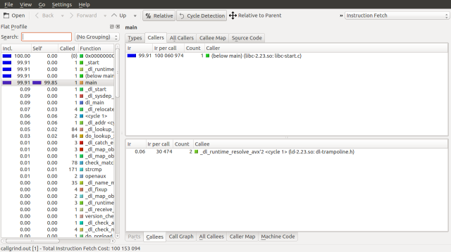
First two basic concepts, starting with an event. Callgrind and Cachegrind (the tool that Callgrind is based on) monitor events that occur within a program. The default event that Callgrind will monitor is called an instruction fetch. When a program is run, its instructions are first loaded into memory. In order to get the next set of instructions that the processor needs it performs an instruction fetch from memory; these events therefore correspond to the lines of code that compose the program.

Callgrind and Cachegrind are capable of monitoring more than just instruction fetches. They can also monitor events like memory cache misses. In our investigation we will be using instruction fetches. You can change the event type used to profile the system using the drop down in the upper right corner or the types tab. Changing the event type will change how the various instructions are costed. See the Cachegrind documentation for more information on events.

The second basic concept is a cycle. A cycle is a group of functions which call each other recursively. Cycles make profiling harder because the code is no longer ordered hierarchically, but the execution of that code is. Certain execution paths may cost more, but accounting for that cost is convolved with other parts of the cycle.

KCachegrind attempts to remove this complexity with a feature called cycle detection. Cycle detection collapses cycles into single blocks and profiles the main branches of the cycle. This feature allows you continue to use the call graph, guided by cost, to find bottlenecks. As we are interested in seeing the structure of the code, we will turn cycle detection off. To toggle cycle detection, press the cycle detection button.

There are a few components of the UI that we can quickly review as well. Back and forward act like a web browser’s history. Up traverses up the call graph. If you go to Settings->Side Bars->Call Stack, you’ll get a “most probable” call stack. Settings->Side Bars->Parts Overview will list different output files if your callgrind command produces multiple outputs. In our case, we will only be examining one output, so this side bar is unnecessary.

By default, KCachegrind will display a Flat Profile on the side bar. This profile displays a global list of functions and their cost. This list can be grouped in a number of ways by going to View->Grouping. In this example we will be using the Flat Profile.

The remaining UI components are found as tabs in the main area of the application. Types is a list of event types available for profiling. The Call Graph is a visualization of the call graph.

Callers are a list of functions that invoke the current function. All Callers are a list looking all the way up the call graph. In a similar manner, Callees and All Callees look down the call graph. The Callee Map looks down the call graph and arranges the proportions of the graph visually. Conversely the Caller Map looks up.

If debugging symbols are enabled, Source Code displays the source for the target function. If the –dump-instr flag is used, then Machine Code will be displayed. We’re not debugging machine code in this investigation.

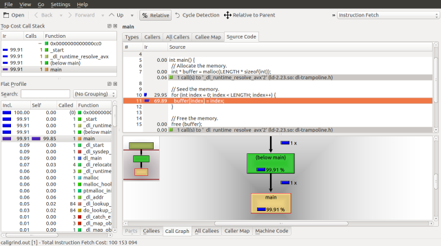
To set up the UI for our investigation, we will want to cost using Instruction Fetch turn off Cycle Detection, view the Source Code and Call Graph tabs, and turn on the Call Stack. Your interface should look like this:

If you misconfigure KCachegrind, you can reset settings by removing the following file:

$ rm ~/.kde/share/config/kcachegrindrc

By taking a look at the source code for our C program above, we can see that the vast majority of time is spent seeding memory. 29.95% of the runtime is spent in the for loop and the remaining 69.89% is spent setting the buffer to the index value.

Before we can get the Python program running with KCacheGrind, we will need to check out the Python source code. The docker container checks out the source code in /tmp and compiles Python with debugging symbols on. In order for our local install of KCacheGrind to be able to access the source, we will need to do the same on our system. Note that you will need to enable your source code repositories in apt for this to work (see System Settings->Software & Updates).

$ cd /tmp
/tmp/$ apt-get source python2.7

Now, on to Python. As in the Massif example, we will have to change ownership of the output file.

src/c/callgrind

src/python/$ cat callgrind
#!/bin/sh
docker run -it -v ${PWD}/results:/results rishiramraj/range_n valgrind --tool=callgrind --callgrind-out-file=/results/callgrind.out ./python -c 'range(10000000)'

src/python/$ ./callgrind
==1== Callgrind, a call-graph generating cache profiler
==1== Copyright (C) 2002-2015, and GNU GPL'd, by Josef Weidendorfer et al.
==1== Using Valgrind-3.11.0 and LibVEX; rerun with -h for copyright info
==1== Command: ./python -c range(10000000)
==1==
==1== For interactive control, run 'callgrind_control -h'.
==1== brk segment overflow in thread #1: can't grow to 0x4a2b000

...

==1== brk segment overflow in thread #1: can't grow to 0x4a2b000
[21668 refs]
==1==
==1== Events    : Ir
==1== Collected : 2899174708
==1==
==1== I   refs:      2,899,174,708

src/python/$ cd results
src/python/results/$ sudo chown $USER:$USER callgrind.out
src/python/results/$ kcachegrind

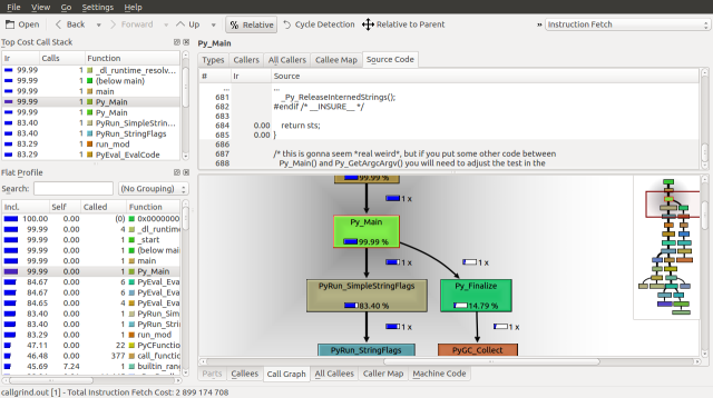
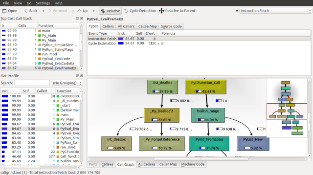
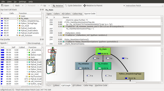
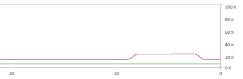
Traversing down the Call Graph, we can see our first fork at Py_Main. 83.4% of the runtime is spent on PyRun_SimpleStringFlags and 14.79% is spent on Py_Finalize. Following the PyRun_SimpleStringFlags branch down we find it splits again at PyEval_EvalFrameEx. A frame is a function call along with its arguments, on the call stack.

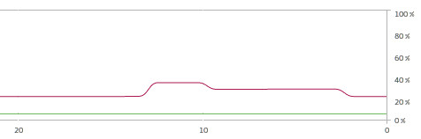
Looking down the Call Graph further, we find that 36.56% of the runtime is spent deallocating our list with the list_dealloc call and 43.32% of the runtime is spent calling the builtin_range function, which creates our list. These functions call _Py_Dealloc and PyInt_FromLong respectfully, which seem to be order n operations, as they are called about 10,000,000 times.

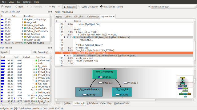
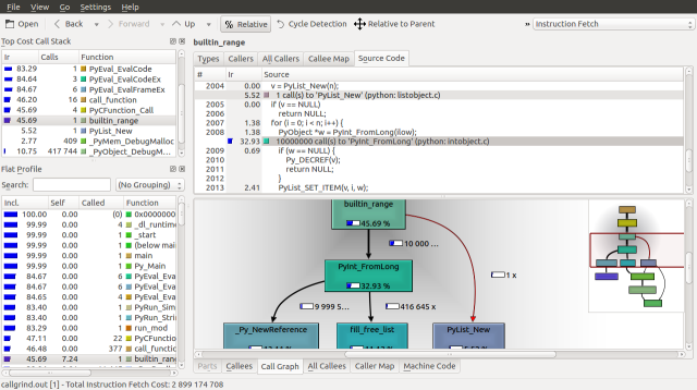
If we inspect the source for builtin_range we can see the PyInt_FromLong and fill_free_list calls, along with how frequently they are called. We can make three observations. The first is that python seems to be maintaining a linked list of objects called free_list. The second is that fill_free_list, which allocates memory according to our Massif analysis is only called only 416,663 times. The third is that the order n operation associated with PyInt_FromLong is the initialization of 9,999,970 PyIntObjects.

Lets dig deeper into this source file to see if we can find the definition for a PyIntObject and the meaning of free_list. I personally use ctags to explore source code, but feel free to use whatever method you feel comfortable with. The definition of a PyIntObject is found in Include/intobject.h, lines 23 to 26:

typedef struct {
    PyObject_HEAD
    long ob_ival;
} PyIntObject;

The definition of the PyObject_HEAD statement is found in Include/object.h on lines 78 to 81:

/* PyObject_HEAD defines the initial segment of every PyObject. */
#define PyObject_HEAD                   \
    _PyObject_HEAD_EXTRA                \
    Py_ssize_t ob_refcnt;               \
    struct _typeobject *ob_type;

It seems that a PyIntObject is an integer that has been wrapped with a reference count and a type. If we look at the source for _Py_NewReference, in Objects/objects.c lines 2223 to 2230, we can see how it is initialized. On the surface, it also seems that the object is added to a global list of objects, but some quick digging (Objects/object.c, lines 40 to 43) suggests that this feature is only enabled when Py_TRACE_REFS is defined. We can likely disregard the 7.61% that is spent on _Py_AddToAllObjects.

void
_Py_NewReference(PyObject *op)
{
    _Py_INC_REFTOTAL;
    op->ob_refcnt = 1;
    _Py_AddToAllObjects(op, 1);
    _Py_INC_TPALLOCS(op);
}

When looking up free_list we find the following comments at the top of Objects/intobject.c on lines 25-30:

/*
block_list is a singly-linked list of all PyIntBlocks ever allocated,
linked via their next members.  PyIntBlocks are never returned to the
system before shutdown (PyInt_Fini).

free_list is a singly-linked list of available PyIntObjects, linked
via abuse of their ob_type members.
*/

Digging deeper into fill_free_list (Objects/intobject.c, lines 47 to 65), we find that integer objects are allocated in blocks and individually linked rear to front using their ob_type:

static PyIntObject *
fill_free_list(void)
{
    PyIntObject *p, *q;
    /* Python's object allocator isn't appropriate for large blocks. */
    p = (PyIntObject *) PyMem_MALLOC(sizeof(PyIntBlock));
    if (p == NULL)
        return (PyIntObject *) PyErr_NoMemory();
    ((PyIntBlock *)p)->next = block_list;
    block_list = (PyIntBlock *)p;
    /* Link the int objects together, from rear to front, then return
       the address of the last int object in the block. */
    p = &((PyIntBlock *)p)->objects[0];
    q = p + N_INTOBJECTS;
    while (--q > p)
        Py_TYPE(q) = (struct _typeobject *)(q-1);
    Py_TYPE(q) = NULL;
    return p + N_INTOBJECTS - 1;
}

The address of the last object in the block is returned and is tracked by the free_list pointer in PyInt_FromLong (Objects/intobject.c, lines 103 to 112).

if (free_list == NULL) {
    if ((free_list = fill_free_list()) == NULL)
        return NULL;
}
/* Inline PyObject_New */
v = free_list;
free_list = (PyIntObject *)Py_TYPE(v);
PyObject_INIT(v, &PyInt_Type);
v->ob_ival = ival;
return (PyObject *) v;

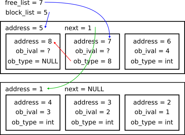
When a new allocation is made, free_list moves forward in the block via its ob_type. The ob_type of the integer object at the beginning of the block is NULL. If free_list is NULL when the next integer is created, a new block is allocated. This process is illustrated below:

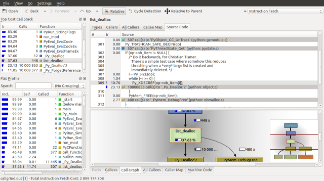
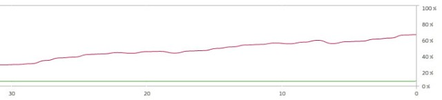
A quick glance at list_dealloc seems to suggest that the bulk of its runtime is spent decreasing reference counts:

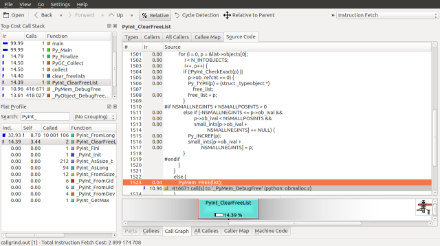
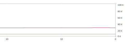
Similarly, a glance at the PyInt_ClearFreeList function, which accounts for the bulk of the Py_Finalize time suggests that the 14.39% of the runtime is spent traversing block_list and free_list to deallocate the memory allocated by fill_free_list.

If we use the detailed snapshot from our Massif example, we can also pinpoint the large list allocation created by PyList_New, which is called from builtin_range. This allocation costs only 5.52% of our runtime. Looking at the source, we can infer that the large memory block contains references to the PyIntObjects created above. These references seem to be set by PyList_SET_ITEM.

KCachegrind will trim the call graph to expose only those functions that have significant cost. If you’re interested in exploring the execution of the interpreter further, you can get interesting insights by reducing the size of the range call to 1,000,000:

src/python/$ docker run -it -v ${PWD}/results:/results rishiramraj/range_n valgrind --tool=callgrind --callgrind-out-file=/results/callgrind.out ./python -c 'range(1000000)'
==1== Callgrind, a call-graph generating cache profiler
==1== Copyright (C) 2002-2015, and GNU GPL'd, by Josef Weidendorfer et al.
==1== Using Valgrind-3.11.0 and LibVEX; rerun with -h for copyright info
==1== Command: ./python -c range(1000000)
==1==
==1== For interactive control, run 'callgrind_control -h'.
==1== brk segment overflow in thread #1: can't grow to 0x4a2b000

...

==1== brk segment overflow in thread #1: can't grow to 0x4a2b000
[21668 refs]
==1==
==1== Events    : Ir
==1== Collected : 347743369
==1==
==1== I   refs:      347,743,369

src/python/$ cd results
src/python/results/$ sudo chown $USER:$USER callgrind.out
src/python/results/$ kcachegrind

Among other things, this profile includes the initialization and module loading code. Unfortunately, that’s an article for another day.

Conclusions

Wow that was a long article, but mystery solved.

Breaking down the runtime of our Python program, we now build an overall picture of how Python allocates and deallocates a large list of integers. Note that this decomposition is based on instruction fetches, and not the actual time spent on each instruction.

• 83.4%: PyRun_SimpleStringFlags
  • 43.32%: builtin_range
    • 5.5%: PyList_New: Allocate a large buffer for the list.
    • 32.92%: PyInt_FromLong
      • 11.13%: fill_free_list: Allocate blocks of memory for integer objects.
      • 13.11%: _Py_NewReference: Set reference counts for integer objects.
  • 36.56%: list_dealloc: Decrease reference counts.
• 14.79%: Py_Finalize: Deallocate integer memory blocks.

The size of n in both cases is 10,000,000 integers. According to Callgrind, the C program used 100,153,094 instruction reads to implement that allocation. The Python program used 2,899,174,708 instruction reads. That’s a ratio of 10:1 instructions per integer in C and 290:1 instructions in Python, in this specific example. In exchange for the additional cycles, Python gives us lists that can be used to contain a range of types and memory management for our integers.

There’s also one very important observation to note from Objects/intobject.c, lines 26, 27:

/*
PyIntBlocks are never returned to the system before shutdown (PyInt_Fini).
*/

This particular observation is noteworthy for long running processes. If you find your process running short on memory, it’s worth checking to see if it allocates a large number of integers.

So what can you do if you need a large list of integers? The easiest solution is to allocate them with a primitive that doesn’t use Python’s memory manager. Available primitives include those from the array module, those from numpy and the multiprocessing.Array primitive for shared memory. You will have to take care to ensure that the process of seeding the memory does not create additional overhead.

With any luck, I’ve been able to successfully introduce you to a set of neat tools and have provided a deeper understanding of how Python manages memory. Practice these skills well, ride the length and breath of the land, and autonomous collectives everywhere will regard your coming favorably.

The Human Rules of Acquisition

There’s very little else as satisfying as calling someone a pataQ, questioning their honour and claiming their D’k tahg. Quoting an obscure rule of acquisition during a business negotiation comes close.

I’ve always found it mildly irritating that humans  don’t have an equivalent. Then I read The Intelligent Investor, by Benjamin Graham and thought “by the Nagus, I’ve found the rules!”

So I highlighted, summarised, summarised again, sorted and then curated the remaining list. I’m a nerd who likes to read text books, what do you want from me?

So, in accordance with the 74th rule of acquisition, “knowledge equals profit”, I present version 0.1.0 of The Rules of Investment:

https://github.com/RishiRamraj/The-Rules-of-Investment/tree/master

Sadly there are only 237 rules 😦 It should go without saying that this is, more or less, an elaborate joke and that if you rely on this summary, you’re insane.

Feel free to shoot me a pull request if you have any other useful rules. For my next trick, I think I’ll translate a Shakespearean play from its original Klingon.

– Qapla’

How To: Make a Dive Knife

Between pizza fuelled coding sessions, I’m occasionally let out to spend time on things that are not programming related. Today I thought; “it’s about time I made a dive knife”, followed by “I may as well blog about it”.

Why Make a Dive Knife?

Diving is a technical field filled with a large number of novices, groups of self taught gurus who tend to do careless things, and a small handful of experts who are dogmatic about the right way of doing things. As a programmer, I fit right in.

With my level of experience I fall well within the novice camp, but as per my usual approach I try to understand and adopt the practices of the expert camp when it’s appropriate. Hopefully I don’t end up falling into the guru camp of divers.

…which brings us to knives. ISE did a recent video about knives and it got me thinking about my own setup. Many divers have a misconception about why they carry a knife. Most of the public seems to think it’s to fend off sharks.

If a shark wants to attack you, about the most effective thing you can do is to blow bubbles; they’re loud and scary. Some divers will carry a bayonet strapped to the inside of their calf thinking they might need to pry open a open a treasure chest.

The reason you carry a dive knife is to cut yourself free from entanglements. Here are two of the most common offenders:

On the left we have mono-filament line, often in the form of nets. On the right we have cave line, which divers usually lay in caves to feel your way out, if you accidentally kick up silt.

So what makes a good dive knife? Here’s a checklist:

• It cuts line.
• It doesn’t cut you, your dry suit, your gloves or  your hoses.
• You can see it when you wear it.
• You can use it with thick gloves on.
• You don’t need to take a yoga class to be able to reach it.

A tiny, blunt knife with a serrated edge fits the bill perfectly. You’d think the diving industry would be able to supply something like that; I suspect they’re hard to sell to the uninitiated.

To be fair, dive rite did introduce the econo knife, which is effectively (if not actually) a ground down steak knife. You can also buy line cutters, which is what I’ve done in the past, but as you’ll see there are limitations. It’s not uncommon for cave and wreck divers to make their own ground down steak knife, diving knives.

Step 0: The Premise

I usually wear two trilobite line cutters near my shoulders (sorry GUE divers, I know it should be on my belt), in two little nylon pouches. I’m going to be taking a little stainless steel serrated knife (above) and turn it into a drop in replacement for a trilobite (below).

Why won’t the trilobite fit all emergency situations? Well, what if a bolt snap gets caught somewhere and I need to cut it free?

Unless I break the plastic guard, it’ll be very hard to get the trilobite to fit in between the bolt snap and the hose. Not a problem for the steak knife:

In addition to the knife, we’ll need some nylon webbing (1 inch), some Velcro and some nylon thread:

A note about thread; it’s common for DIYers to use great materials for everything except the thread, only to find their creations unravelling when used. Here’s the stuff that I use, via ebay:

Step 1: Grind Down the Blade

For want of a bench grinder, I opted to use my Dremel with a diamond cutoff wheel to cut the profile of the blade.

Knives have a temper, which means that the metal has been heated to a certain temperature which causes the steel to have a certain hardness (I’m not a metallurgist). If you overheat the steel (say by attacking it with a diamond cutoff wheel), you may end up ruining the temper. So I occasionally dunked the blade into a cup full of water. I’m not sure if it actually helps.

After some coaxing with some grinding stones, I finally had the blade profile I wanted.

Step 2: Cut the Handle

Next, it was time to introduce the knife to the band saw in order to cut the handle down to size.

Fortunately this knife wasn’t a full tang knife (you can check with a strong light). Here’s the knife cut down to size:

I then drilled a hole to attach the Velcro strip, and shaped the hole using a grinding attachment.

Step 3: Create the Velcro Strap

With the knife done, it’s time to focus on the Velcro strap. The strap serves two purposes. It allows you to store the knife securely in its nylon sheath. It also acts as an extended handle. First, I started with a loop:

Then I sandwiched the loop in between two strips of Velcro.

Finally, I attached the knife to the strap using a bit of cave line. ISE has a video on tying off gear.

All Done

I present the finished knife:

A quick neoprene glove test:

And the knife mounted on my back plate, well within eye shot, deploy-able with a single hand.

Python vs Copy on Write

I recently found myself awake at 4 AM trying to science myself out of a memory problem in Python on Linux. If you’re trying to share a read only cache to a number of Linux subprocesses and find yourself running out of memory and time, this blog is for you. The tl;dr of the story is down below.

This issue was the first serious whack I’ve had at tuning memory issues in Python. I’m by no means an expert on the subject so feel free fill in some of the gaps in the comments below.

For the purposes of this blog, I’ll try to keep the toolset simple. No fancy valgrind, just Stock Python 2.7 scripts running on Ubuntu 15.04, with some PyPy thrown in for bonus points. I’ll be allocating a bunch of memory and hoping it shows up in the stock Ubuntu System Monitor.

There are most certainly better tools available. If you’re running in production, you’ll want to log the memory consumption of your process and have a way of associating it with what is happening in your process. Be sure to keep some Linux performance tools tucked safely under your pillow, as well as some grep, awk, sed and gnuplot goodness for log file mining.

However, instead of tooling I’d like to talk basic concepts. It’s important to understand the mechanics of a problem before trying to treat it, and that’s what I hope to accomplish with this blog. With that said, let’s dive into the problem.

Measure First

The bit of code I was trying to tune was a basic multiprocessing worker pool running on Linux (i.e. using fork). The code will fork, do some processing and join the main process when its complete. Each worker in the pool requires a cache of data to do its job. Those familiar with copy on write issues in Python will immediately spot the problem. I’ll go over details of this problem in the section below.

However, I should underscore that when you’re dealing with performance issues, a large part of the effort is properly diagnosing the problem. As with any performance issue, the size of n matters just as much as the code that processes it. While I had suspicions that my problem was a copy on write issue, I did not pursue a solution until I had clear evidence that suggested my hypothesis.

Like unit testing, this sort of rigour grows more important as time lines shrink…which begs the question, how do you know you have a memory issue? Or more specifically:

On Linux, oom-killer (out of memory) is lurking in the background waiting to defend your system from processes that request too much memory. Unfortunately you will loose your traceback because the process will be halted and won’t be given the opportunity to generate a traceback. If you ever find yourself wondering why your Python process abruptly halted, check your syslog for something like:

Jan 24 00:00:23 host kernel: python invoked oom-killer: gfp_mask=0x100bc, order=0, oom_adj=0, oom_score_adj=0

So, hopefully you’ve done your diligence and come to the conclusion that you have a memory issue associated somehow with multiprocessing. What’s next?

The Problem

I was fortunate to be sitting in the audience when Brandon Rhodes gave his talk on Python, Linkers, and Virtual Memory at PyCon. He does a much better job of explaining Copy on Write than I do in this blog, so go watch the video. I’ll try to do a quick summary of his talk here, so that you can understand all of the working pieces.

A very simple mental model for memory is a list of data blocks that each have an address. “How much memory does a process use?” is a loaded question for the simple reason that processes share memory.

If two processes want to load the same shared library, instead of loading the library into two separate addresses, the operating system can load it into one address and point both processes to the same address in memory. As a result there is a distinction between the total memory actually used by a process (called the Resident Set Size or RSS) and the virtual memory used by a process (called the Virtual Memory Size or VMS).

In addition to sharing code, processes can also share data. The classic example on Unix happens when forking a child process. When you fork a child process on Unix, it doesn’t re-run the process from scratch. Instead it will create a new process and point the processes virtual memory to the same physical blocks that the parent is using.

This practice works well until until either process needs to modify the memory. When this happens, the operating system will create a copy of the memory block and then write the data; hence the term copy on write.

Copy on write is handy for creating caches that subprocesses can reference. The reason is because read only memory need only be referenced, and not actually duplicated, significantly reducing the memory overhead of a subprocess.

Copy on write is a problem for Python because its objects are reference counted. To keep track of when an object should be deleted, Python stores a count of how many references to an object currently exist. When that count reaches 0 the object can be cleaned. Benjamin Peterson has an interesting talk on the subject.

The unfortunate implication is that when your subprocess comes along, even the act of reading a block of memory will result in a duplicate copy of the data being created as Python needs to update the reference count.

As a result, every new subprocess that reads the cache will also create a full copy of the cached data.

The Benchmark

WARNING: Running some of these tests might run your computer out of memory and possibly crash it or worse. Here be dragons. Use proper precautions.

Before we dive into a full blown solution, we’ll need a benchmark for comparison. If we can address the behaviour we see in the benchmark, we’ve got a candidate solution.

The benchmark is relatively simple. It first creates a large data structure to serve as our cache using the range function with a very large number. It will then spawn a number of subprocesses that attempt to read from the cache. The expectation is that our memory usage will be multiplied by the number of subprocesses that we spawn.

In order to run these examples, you’ll have to tune them a bit to get them to show up in your system monitor. Three parameters control the behaviour of the benchmark script below. The most important is the CACHE, which specifies the number of records to be created (i.e. the very large number above). PROCESSES is the number of subprocesses that we’ll spawn. To differentiate between the cache allocation part of the benchmark and the subprocess part, we’ll inject a number of pauses using PAUSE, in seconds.

Tuning CACHE can be a bit tricky. In order to reproduce my experiments you’ll need the process to show up distinctly in your system monitor. Again take caution because running your machine out of memory is easier than you think. I’ve intentionally made the CACHE size small enough for most machines. I usually add 0s to the CACHE size until it consumes about 5% of the memory on the machine. Setting the PAUSE value to something low will also speed up this process.

Here’s the benchmark:

#!/usr/bin/env python
# -*- coding: utf-8 -*-

from multiprocessing import Pool
from time import sleep

# The size of the cache created when calling range(CACHE). To ensure that your
# processes is visible on your system, you will need to adjust this value.
# Start with the CACHE value below and keep adding 0s until anywhere between
# 5-10% of your memory is consumed. You may also want to reduce the PAUSE
# value below to make this tuning easier. Note that IT IS VERY EASY TO RUN
# YOUR SYSTEM OUT OF MEMORY THIS WAY, so save everything before attempting.
CACHE = 10000

# The number of subprocesses forked.
PROCESSES = 5

# The number of seconds to pause in order to display the allocated memory in
# the system monitor.
PAUSE = 3

def job(cache):
    '''
    An artificial job that sleeps for a second and then reports memory usage.
    '''
    # Read all of the data in the cache. Note that in order to see the effect
    # the copy on write problem, we need to actually read the cache. By reading
    # the cache, we create a new reference to the memory being tracked and
    # therefore copy the memory although all we're doing is reading.
    for item in cache:
        pass

    # Make sure the memory that the allocated memory is visible in the system
    # monitor.
    sleep(PAUSE)

def main():
    '''
    Entry point.
    '''
    # Create the cache. Note that allocating a large amount of memory takes
    # time. After the memory is allocated, we want to make sure the new memory
    # level is visible in the system monitor, so we pause.
    cache = range(CACHE)
    sleep(PAUSE)

    # Run the jobs.
    pool = Pool(PROCESSES)
    pool.map(job, [cache]*PROCESSES)

if __name__ == '__main__':
    main()

Here’s what happens when we run the benchmark:

Time proceeds from left being the start to right being the end. You can see the first long PAUSE after the cache is allocated. Then the cache is magnified and the second long PAUSE caused by the parallel processes all finishing.

The Solution?

The core of our solution is to tell the operating system that it should be using shared memory that isn’t reference counted. Fortunately, multiprocessing has a number of primitives that can help. Unfortunately, there are a few ways to use these primitives and some of them have pitfalls.

Note that some of this section will be conjecture on my part. I’ll try to probe as deep as I can, but some of this material will have to be left for later blogs.

The first consideration is how we launch and manage our subprocesses. In particular, weather we should use multiprocessing.Pool.map or multiprocessing.Process to launch our subprocess. Sadly it matters.

The second consideration is speed. If we’re not careful and use the wrong primitives, we may pay a runtime cost. As we are attempting to produce a read only cache, we’re going to try to optimize both the memory consumption and runtime of our code.

Something That Works

Our first priority is to get something that works as painlessly as possible to confirm the core premise; that shared memory will fix our problem. We can bypass a lot of complexity by using a global object.

Note that to address our second concern, we need to tell the array not to lock. Once launched, all of our jobs will start reading immediately and if the cache locks, our subprocesses will all contend for read access; we won’t get any benefit from parallelism.

Setting lock to False is generally a bad idea if you have writes into your cache from a separate subprocess. However if you prepare the cache in advance and only read from it in your subprocesses, you should be okay.

Feel free to set lock=True if you like, but be prepared for a long runtime and keep the kill command handy.

#!/usr/bin/env python
# -*- coding: utf-8 -*-

from multiprocessing import Pool, Array
from time import sleep

# The size of the cache created when calling range(CACHE). To ensure that your
# processes is visible on your system, you will need to adjust this value.
# Start with the CACHE value below and keep adding 0s until anywhere between
# 5-10% of your memory is consumed. You may also want to reduce the PAUSE
# value below to make this tuning easier. Note that IT IS VERY EASY TO RUN
# YOUR SYSTEM OUT OF MEMORY THIS WAY, so save everything before attempting.
CACHE = 10000

# The number of subprocesses forked.
PROCESSES = 5

# The number of seconds to pause in order to display the allocated memory in
# the system monitor.
PAUSE = 3

# A global object that contains the generated cache.
cache = None

def job(arg):
    '''
    An artificial job that sleeps for a second and then reports memory usage.
    '''
    # Read all of the data in the cache. Note that in order to see the effect
    # the copy on write problem, we need to actually read the cache. In this
    # case the problem doesn't happen because cache is an Array object, which
    # lives in shared memory.
    global cache
    for item in cache:
        pass

    # Wait for the system monitor.
    sleep(PAUSE)

def main():
    '''
    Entry point.
    '''
    # Create a global shared memory cache to address the copy on write issue.
    # We need to tell the array not to lock. All of our jobs will start reading
    # immediately from the cache and if the array locks, our subprocesses will
    # all contend for read access.
    global cache
    cache = Array('i', range(CACHE), lock=False)
    sleep(PAUSE)

    # Run the jobs.
    pool = Pool(PROCESSES)
    pool.map(job, [None]*PROCESSES)

if __name__ == '__main__':
    main()

Running the script, it looks like we have a winner:

Now that we have something that works, let’s see if we can make it any better. Using a global variable is bad because of the large potential for import side effects that come with it. Next, we’ll see if we can pass the cache as a parameter.

Consideration the First: Pool vs Process

Why is process management a consideration? Intuitively, when I started hacking on this problem, I expected that both Pool.map and Process to work in approximately the same way. Let’s see what happens if we attempt to take the example above and pass the shared memory cache as a parameter to map.

#!/usr/bin/env python
# -*- coding: utf-8 -*-

from multiprocessing import Pool, Array
from time import sleep

# The size of the cache created when calling range(CACHE). To ensure that your
# processes is visible on your system, you will need to adjust this value.
# Start with the CACHE value below and keep adding 0s until anywhere between
# 5-10% of your memory is consumed. You may also want to reduce the PAUSE
# value below to make this tuning easier. Note that IT IS VERY EASY TO RUN
# YOUR SYSTEM OUT OF MEMORY THIS WAY, so save everything before attempting.
CACHE = 10000

# The number of subprocesses forked.
PROCESSES = 5

# The number of seconds to pause in order to display the allocated memory in
# the system monitor.
PAUSE = 3

def job(cache):
    '''
    An artificial job that sleeps for a second and then reports memory usage.
    '''
    # Read all of the data in the cache.
    for item in cache:
        pass

    # Wait for the system monitor.
    sleep(PAUSE)

def main():
    '''
    Entry point.
    '''
    # Create a shared memory cache.
    cache = Array('i', range(CACHE), lock=False)
    sleep(PAUSE)

    # Run the jobs.
    pool = Pool(PROCESSES)
    # At this point, cache is expected to break the map function, because map
    # attempts to pickle the iterate parameter.
    pool.map(job, [cache]*PROCESSES)

if __name__ == '__main__':
    main()

When we run above we get the following traceback:

Traceback (most recent call last):
 File "./map.py", line 52, in <module>
 main()
 File "./map.py", line 48, in main
 pool.map(job, [cache]*PROCESSES)
 File "/usr/lib/python2.7/multiprocessing/pool.py", line 251, in map 
 return self.map_async(func, iterable, chunksize).get()
 File "/usr/lib/python2.7/multiprocessing/pool.py", line 567, in get 
 raise self._value
cPickle.PicklingError: Can't pickle <class 'multiprocessing.sharedctypes.c_int_Array_10000000'>: attribute lookup
 multiprocessing.sharedctypes.c_int_Array_10000000 failed

It seems like map is trying to pickle our Array primitive. If I had to guess, it’s trying to store the elements of the iterable in a queue and failing. Let’s see what happens if we try to use multiprocessing.Process (multirpocessing.Manager is discussed below):

#!/usr/bin/env python
# -*- coding: utf-8 -*-

from multiprocessing import Process, Array
from time import sleep

# The size of the cache created when calling range(CACHE). To ensure that your
# processes is visible on your system, you will need to adjust this value.
# Start with the CACHE value below and keep adding 0s until anywhere between
# 5-10% of your memory is consumed. You may also want to reduce the PAUSE
# value below to make this tuning easier. Note that IT IS VERY EASY TO RUN
# YOUR SYSTEM OUT OF MEMORY THIS WAY, so save everything before attempting.
CACHE = 10000

# The number of subprocesses forked.
PROCESSES = 5

# The number of seconds to pause in order to display the allocated memory in
# the system monitor.
PAUSE = 3

def job(cache):
    '''
    An artificial job that sleeps for a second and then reports memory usage.
    '''
    # Read all of the data in the cache.
    for item in cache:
        pass

    # Wait for the system monitor.
    sleep(PAUSE)

def main():
    '''
    Entry point.
    '''
    # Create a global shared memory cache.
    cache = Array('i', range(CACHE), lock=False)
    sleep(PAUSE)

    # Run the jobs using Process and not map.
    for index in range(PROCESSES):
        process = Process(target=job, args=(cache, ))
        process.start()

if __name__ == '__main__':
    main()

When we run the script:

That works but by switching to Process, we’ve given up a lot of the nice functionality that we get with map. Fortunately, multiprocessing has a solution for this problem in the form of multiprocessing.Manager. Manager is a class that will wrap data structures in proxies that can then be pickled.

Taking a look at the configuration it seems as though the manager should work. However, the manager does not respect the lock parameter and so if you do dare to run the script below, prepare yourself for a long runtime.

WARNING: I do not recommend running the script below. It has a long runtime.

#!/usr/bin/env python
# -*- coding: utf-8 -*-

from multiprocessing import Pool, Manager
from time import sleep

# The size of the cache created when calling range(CACHE). To ensure that your
# processes is visible on your system, you will need to adjust this value.
# Start with the CACHE value below and keep adding 0s until anywhere between
# 5-10% of your memory is consumed. You may also want to reduce the PAUSE
# value below to make this tuning easier. Note that IT IS VERY EASY TO RUN
# YOUR SYSTEM OUT OF MEMORY THIS WAY, so save everything before attempting.
CACHE = 10000

# The number of subprocesses forked.
PROCESSES = 5

# The number of seconds to pause in order to display the allocated memory in
# the system monitor.
PAUSE = 3

def job(cache):
    '''
    An artificial job that sleeps for a second and then reports memory usage.
    '''
    # Read all of the data in the cache.
    for item in cache:
        pass

    # Wait for the system monitor.
    sleep(PAUSE)

def main():
    '''
    Entry point.
    '''
    # Create a shared memory cache using a memory manager. Unfortunately this
    # manager doesn't seem to respect the lock=False argument, causing a lot
    # of reading contention and therefore a long runtime.
    manager = Manager()
    cache = manager.Array('i', range(CACHE), lock=False)

    # Run the jobs.
    pool = Pool(PROCESSES)
    pool.map(job, [cache]*PROCESSES)

if __name__ == '__main__':
    main()

As it stands, I’m not sure if this is a bug. multiprocessing does allow for some extensibility, however I’ve yet to figure out the right song and dance to make it all work. If there’s interest, I can do a deep dive into the guts of multiprocessing in another blog.

No Read?

As an aside, what happens if we comment out the following lines?

 for item in cache:
     pass

If our theory is correct, then Python will not have to build references to the individual records in the cache, and the memory will not be copied. Note that this trick will only work in the Process version because the Pool.map version will always pickle the memory.

#!/usr/bin/env python
# -*- coding: utf-8 -*-

from multiprocessing import Process
from time import sleep

# The size of the cache created when calling range(CACHE). To ensure that your
# processes is visible on your system, you will need to adjust this value.
# Start with the CACHE value below and keep adding 0s until anywhere between
# 5-10% of your memory is consumed. You may also want to reduce the PAUSE
# value below to make this tuning easier. Note that IT IS VERY EASY TO RUN
# YOUR SYSTEM OUT OF MEMORY THIS WAY, so save everything before attempting.
CACHE = 10000

# The number of subprocesses forked.
PROCESSES = 5

# The number of seconds to pause in order to display the allocated memory in
# the system monitor.
PAUSE = 3

def job(cache):
    '''
    An artificial job that sleeps for a second and then reports memory usage.
    '''
    # With these lines omitted, the copy on read issue won't occur because
    # python will not build references as a result of reading the memory.
    '''
    for item in cache:
        pass
    '''

    # Wait for the system monitor.
    sleep(PAUSE)

def main():
    '''
    Entry point.
    '''
    # Create a global shared memory cache.
    cache = range(CACHE)
    sleep(PAUSE)

    # Run the jobs using Process and not map.
    for index in range(PROCESSES):
        process = Process(target=job, args=(cache, ))
        process.start()

if __name__ == '__main__':
    main()

As expected, no cache duplication:

Consideration the Second: Speed

If our cache is large, then accessing it needs to be fast. We’ve already tackled part of this problem by setting lock=False above, with the assumption that the cache will be read only. That takes care of the issues associated with subprocesses contending for read. Now we’ll look at the process of getting the data from the Array into the Python subprocess.

Time for more speculation on my part. Under the hood, Array is actually a primitive C array allocated with malloc. When the Python subprocess iterates over this array, it creates an internal Python integer, which takes time.

Wouldn’t it be handy if we could just read directly from the buffer? numpy to the rescue with the frombuffer function. This function takes our Array and reads directly off it from the blocks in memory. First lets install numpy in a virtualenv:

 $ mkvirtualenv numpy
 $ pip install numpy

Then let’s run the example:

#!/usr/bin/env python
# -*- coding: utf-8 -*-

from multiprocessing import Process, Array
from time import sleep
import numpy

# The size of the cache created when calling range(CACHE). To ensure that your
# processes is visible on your system, you will need to adjust this value.
# Start with the CACHE value below and keep adding 0s until anywhere between
# 5-10% of your memory is consumed. You may also want to reduce the PAUSE
# value below to make this tuning easier. Note that IT IS VERY EASY TO RUN
# YOUR SYSTEM OUT OF MEMORY THIS WAY, so save everything before attempting.
CACHE = 10000

# The number of subprocesses forked.
PROCESSES = 5

# The number of seconds to pause in order to display the allocated memory in
# the system monitor.
PAUSE = 3

def job(cache):
    '''
    An artificial job that sleeps for a second and then reports memory usage.
    '''
    # Read all of the data in the cache.
    for item in numpy.frombuffer(cache, 'i'):
        pass

    # Wait for the system monitor.
    sleep(PAUSE)

def main():
    '''
    Entry point.
    '''
    # Create a global shared memory cache.
    cache = Array('i', range(CACHE), lock=False)
    sleep(PAUSE)

    # Run the jobs.
    for index in range(PROCESSES):
        process = Process(target=job, args=(cache, ))
        process.start()

if __name__ == '__main__':
    main()

When compared to the vanilla approach, we get a marginal improvement on the subprocess runtime. As n grows, this margin should grow as well. As always, your mileage may vary:

It is also possible to do all of this magic with strings, however be cautioned that the Array object must be both written and read with a fixed character length. Brush up on your malloc skills and you should be just fine.

tl;dr

If you’re looking for a vanilla example, look here:

#!/usr/bin/env python
# -*- coding: utf-8 -*-

from multiprocessing import Process, Array
from time import sleep

# The size of the cache created when calling range(CACHE). To ensure that your
# processes is visible on your system, you will need to adjust this value.
# Start with the CACHE value below and keep adding 0s until anywhere between
# 5-10% of your memory is consumed. You may also want to reduce the PAUSE
# value below to make this tuning easier. Note that IT IS VERY EASY TO RUN
# YOUR SYSTEM OUT OF MEMORY THIS WAY, so save everything before attempting.
CACHE = 10000

# The number of subprocesses forked.
PROCESSES = 5

# The number of seconds to pause in order to display the allocated memory in
# the system monitor.
PAUSE = 3

def job(cache):
    '''
    An artificial job that sleeps for a second and then reports memory usage.
    '''
    # Read all of the data in the cache.
    for item in cache:
        pass

    # Wait for the system monitor.
    sleep(PAUSE)

def main():
    '''
    Entry point.
    '''
    # Create a global shared memory cache.
    cache = Array('i', range(CACHE), lock=False)
    sleep(PAUSE)

    # Run the jobs using Process and not map.
    for index in range(PROCESSES):
        process = Process(target=job, args=(cache, ))
        process.start()

if __name__ == '__main__':
    main()

If you’re using numpy, look here:

#!/usr/bin/env python
# -*- coding: utf-8 -*-

from multiprocessing import Process, Array
from time import sleep
import numpy

# The size of the cache created when calling range(CACHE). To ensure that your
# processes is visible on your system, you will need to adjust this value.
# Start with the CACHE value below and keep adding 0s until anywhere between
# 5-10% of your memory is consumed. You may also want to reduce the PAUSE
# value below to make this tuning easier. Note that IT IS VERY EASY TO RUN
# YOUR SYSTEM OUT OF MEMORY THIS WAY, so save everything before attempting.
CACHE = 10000

# The number of subprocesses forked.
PROCESSES = 5

# The number of seconds to pause in order to display the allocated memory in
# the system monitor.
PAUSE = 3

def job(cache):
    '''
    An artificial job that sleeps for a second and then reports memory usage.
    '''
    # Read all of the data in the cache.
    for item in numpy.frombuffer(cache, 'i'):
        pass

    # Wait for the system monitor.
    sleep(PAUSE)

def main():
    '''
    Entry point.
    '''
    # Create a global shared memory cache.
    cache = Array('i', range(CACHE), lock=False)
    sleep(PAUSE)

    # Run the jobs.
    for index in range(PROCESSES):
        process = Process(target=job, args=(cache, ))
        process.start()

if __name__ == '__main__':
    main()

PyPy

Time for some bonus points. pypy is awesome and weird in all of the ways that make my mad scientist senses tingle. One of those ways is its pluggable garbage collection system.

The default collector is called minimark. I know very little about pypy, but I’ll try to give a quick overview. See Benjamin Peterson’s talk for more detail.

The underlying algorithm is called Mark and Sweep. It cleans memory in two phases. In the first phase, it will walk the reference tree and mark objects that are still alive. In the second phase it will sweep away any objects that aren’t marked. As a result no reference counting, which means copy on write should work out of the box.

Let’s test it! First, let’s install pypy and create our virtualenv:

$ sudo apt-get install pypy
$ mkvirtualenv -p /usr/bin/pypy pypy

Now let’s rerun the benchmark with no changes and see what happens:

So, that’s not exactly what we expected. I suspect pypy doesn’t like the pickling that needs to happen to get the cache into Pool.map. Let’s tweak the code to use Process instead, except without Array:

#!/usr/bin/env python
# -*- coding: utf-8 -*-

from multiprocessing import Process
from time import sleep

# The size of the cache created when calling range(CACHE). To ensure that your
# processes is visible on your system, you will need to adjust this value.
# Start with the CACHE value below and keep adding 0s until anywhere between
# 5-10% of your memory is consumed. You may also want to reduce the PAUSE
# value below to make this tuning easier. Note that IT IS VERY EASY TO RUN
# YOUR SYSTEM OUT OF MEMORY THIS WAY, so save everything before attempting.
CACHE = 10000

# The number of subprocesses forked.
PROCESSES = 5

# The number of seconds to pause in order to display the allocated memory in
# the system monitor.
PAUSE = 3

def job(cache):
    '''
    An artificial job that sleeps for a second and then reports memory usage.
    '''
    # Read all of the data in the cache.
    for item in cache:
        pass

    # Wait for the system monitor.
    sleep(PAUSE)

def main():
    '''
    Entry point.
    '''
    # Create a global shared memory cache.
    cache = range(CACHE)
    sleep(PAUSE)

    # Run the jobs using Process and not map.
    for index in range(PROCESSES):
        process = Process(target=job, args=(cache, ))
        process.start()

if __name__ == '__main__':
    main()

Now that’s the kind of result that makes me smile 🙂 And yes, I did check to make sure that the process actually ran :p

Results

After running the patched code in production, I’m happy to report that it worked. Huzzah for science!

As a general rule it’s hard to gauge the performance of a patch until you run it in production. In this particular case, I had good evidence to suggest the root cause of the problem and the memory was reduced to the bottleneck I predicted.

We also got a bit of runtime back, but that’s a story for a future blog. I’d also like to do a deeper dive into Python’s memory allocation and see if we can break out strace and valgrind.

Until then, if you’re stuck on a hard problem just remember, try science!

Explaining Technical Debt

I’ve been thinking about technical debt and how it builds in software projects. Brace yourself, this is a depressing topic so I’ve included a picture of a turtle. Hopefully that makes you feel better.

Good? Good.

It’s very easy to come up with a specific example of technical debt and then say, if we fixed that problem the project would be much easier to modify and therefore cheaper to maintain. The real trouble with technical debt is explaining how important it is to someone without a technical background. As a rule, it’s very easy to justify the next great feature in terms of sales. It’s a measurable win and makes everyone very happy very fast.

Technical debt, true to it’s name, is another beast entirely. It builds up slowly over time. Everyone knows it’s there and can see the disease spreading but it isn’t until it’s too late that you can convince people to take action. It’s too late when you need to rewrite your software to add the next essential feature. For the economically literate, this is when your marginal cost exceeds your marginal revenue.

The end result is a long and gruelling recovery in the best case and shutting down the business in the worst. There’s nothing much that can be done about the temptation to trade long term cost savings for short term revenue. But with a useful analogy we may be able to shed some light on the dragon lurking in the darkness of the treasure cave.

Technical debt is very much like debt, but with a different currency. In the world of software we trade time for features. In an ideal world, the cost of a feature is static. It doesn’t matter if you implement the feature this cycle or five years from now, it costs the same amount of time. This is probably how management thinks software development works. They’ll probably also get confused when that’s no longer the case.

Now let’s add a bit of complexity. Your boss asks for a feature that is kinda pricey for this cycle. Normally you’d tell them no, but instead you decide to borrow some time from the next release by cutting corners. You’re hailed as a technical hero for meeting the deadline. You think to yourself, things will be okay if you spend a bit of time next release to pay back the time you borrowed.

However, now you’ve set a precedent and the credit genie is out of the bottle. The next release comes along and again you’re strapped for time and so you borrow more time. This time it’s only moderately worse so again you figure you’ll spend an all nighter or two to get it done right in the next release.

Unfortunately, debt compounds over time. When the debt is low the problem is small but when the debt is high, no amount of all nighters during a release can help you. What you need to do is spend some serious time paying down the debt by fixing the small compromises you’ve made over past releases.

Up to this point, you’ve hit all of your deadlines. How do you tell management that we need to spend a whole cycle rewriting code that already works? The reality is that it’s already getting too late because if you try to add features this release, it wil get worse. Instead let’s look at what we can do before things spin out of control.

Do you necessarily have to borrow? If you put together a killer team and invest heavily on testing you’ve solved the problem right? Well, not really. Any sufficiently complex project has unexplored problems and your project team needs to learn the best ways to solve these problems. That often means borrowing refactoring time from the future to try something new today.

But having a killer team helps, right? It does, but not in the way you might think. It doesn’t reduce your overall debt as that is really part of your source code. Having a good team is like having a credit card with a cheap interest rate. You can borrow less time from future releases with clever solutions today, but you’re still borrowing. If you’ve already accumulated debt in your source code, you still need to pay that debt no matter which team you have.

Sometimes you get lucky and a good developer will find a clever solution to a core problem that clears a bunch of debt. Sometimes you get unlucky and you’ll find that you’ve accidentally built your software on a mud bank that is washing away.

Anomalies aside, the place to be is where you can service your debt. That is, you are clearing enough of it to keep the amount of time between releases to an acceptable level. If the time between releases starts to go up quickly over every release, you’ve got a problem. It’s time to stop and refactor.

Good teams refactor constantly and are always assessing whether their designs fit their requirements. The rule of thumb I’ve seen thrown around is about one developer on one refactoring task per cycle per 5-10 developers. This number will depend very much on your industry and quality requirements.

So let’s summarise the analogy. Building software is like spending time for features. Sometimes you have to borrow time from a future release to buy a feature. If you do, your team determines the interest rate you have to pay and your source code is your balance sheet. If you don’t pay back your debt, you will no longer be able to modify your software and bad things will happen.

The scariest part is that most management teams are often spending credit as though there were no interest rates. The only people that can warn them are the engineers, so it’s time to start complaining. Your weekends depend on it.

sqlpyzer: IPython + sqlite in html5

What is a sqlpyzer?

sqlpyzer is an experimental plugin I wrote for the IPython  Notebook. It’s much easier to describe what it is in a video, so here goes:

You can find the source and the installation instructions here:

https://github.com/RishiRamraj/sqlpyzer

The Name

Sadly all of the good SQL names were taken. I was going for sqlizer but things fell apart quickly when I tried to add py.

Installation

There are installation instructions on the github page, but I’ll go into a bit more detail here. I haven’t tested these steps, so please comment with any corrections. I’m currently running Ubuntu 12.04 32bit desktop. I’ve tested the plugin using Python 2.7 and Chromium. I’m going to assume that you have your github repository located in ~/Repo. You’ll need a specific build of IPython; one that supports jsplugins. You can find such a build at:

https://github.com/RishiRamraj/ipython

Be sure to check out the “json” branch. Once you have ipython checked out you can then run the notebook by using the ipython.py script in the root directory. This script will then launch the notebook and open a browser.

user@computer:~/Repo/ipython$ python ipython.py notebook

Next, we’ll install sqlpyzer (again, sorry for the name). Close the notebook for now, we’ll get back to it later. I recommend you use pip and virtualenv. If you’re not familiar with these tools, check this out:

http://jontourage.com/2011/02/09/virtualenv-pip-basics/

Install sqlpyzer:

user@computer:~/Repo/sqlpyzer$ pip install -e .

By using a develop egg above, you’ll be able to modify sqlpyzer without having to reinstall it. Next, we’ll have to install the sqlpyzer javascript. You’ll need to find the ipython local configuration folder. In Ubuntu:

user@computer:~$ cd .config/ipython/profile_default/static/jsplugins/

Simlink the Javascript files so that you can modify the Javascript in your repository:

user@computer:~/.config/ipython/profile_default/static/jsplugins% ln -s /home/user/Repo/sqlpyzer/js/* .

Finally, run the notebook again and open the notebook located here to test the plugin:

~/Repo/sqlpyzer/sqlpyzer.ipynb

Repo Structure

There are three things of interest in the sqlpyzer repo. The sqlpyzer folder contains all of the python responsible for getting the data out of python and marshalled into json. The js folder contains all of the javascript that creates the sqlite database and marshals the json into the database.

Python

load.py

The load.py module contains one function. It is called by the load_ext function in IPython. Its job is to tell IPython how to take a data object and display it. Everything comes together on this line:

formatter.for_type_by_name(module, name, serializer)

The serializer function is called every time you issue the display command on a sqlpyzer.Data object.

data.py

This module contains a simple validator and data type. Besides validation, the only real purpose this data type servers is to be able to associate Data objects with a specific serializer function that tells IPython which Javascript handler to use.

serialize.py

The function in this module turns the Data object into a json string. The resulting object has two properties. First is the data object. Note that the “data” key can really be called anything. Second is the handler. The handler is special as it tells IPython which Javascript function to use to interpret the json being passed in.

__init__.py

In order for IPython to be able to load a module as an extension, the module needs to have a load_ipython_extension function. The __all__ list tells python that it should load the load_ipython_extension when the module is loaded, as an attribute of the module. If you’re not familiar with __all__, take a look at:

http://docs.python.org/2/tutorial/modules.html#importing-from-a-package

Everything Else

constants.py has some constants like the Javascript callback name. test.py contains tests. To run the tests use:

user@computer:~/Repo/sqlpyzer/sqlpyzer$ python test.py

Javascript

Disclaimer: I know more about Python than I do Javascript.

console.js

Ths script takes the id of a div as an argument, and creates the database object with the UI. The UI should automatically resize its controls to fit in whatever container you put it in. The display function is the interesting part in this module. It demonstrates how to retrieve data from a sqlite query. Once the console is created, it returns an object containing the database, input and output fields.

sqlpyzer.js

Possibly the largest single piece of source in this project. If you’re looking for the Javascript that associates a the handler name with the Javascript callback, look all the way at the end of the file:

IPython.json_handlers.register_handler('sqlpyzer_data', sqlpyzer.data);

The sqlpyzer.data callback takes two parameters; the json object that we serialised in from python and the new element created under the display function. It then creates a console and uses the json data to populate the database.

When reading the create_table code, it’s important to remember that Javascript doesn’t block when executing SQL. Instead, you need to specify callbacks that are called if a query succeeds or fails. You can get away with calling them in parallel in a single transaction, if your queries are independent as with this for loop. In the background, javascript is queuing the SQL execution to happen as a set of callbacks, once the for loop is complete.

// Create all the tables.
console.database.transaction(function (tx) {
     for (table in json.data) {
         sqlpyzer.create_table(tx, table, json.data[table]);
     } 
});

If your queries depend on other queries like row insertion depending on table creation, things start getting interesting. You need to specify a callback that will insert all of the rows once the table has been created. You’ll notice that the create_table function has two functions called create_schema and insert_row for this reason. create_schema exposes a callback called next that then inserts all of the rows in parallel:

// Pull it all together to create the table.
create_schema(tx, function(tx) {
    for (var index = 0; index < table.length; index++) {
        var row = table[index];
        insert_row(tx, row);
    }
});

Closures make this sort of work a easy. They basically set the context for the callbacks used to create the schema and the individual rows. Otherwise, we would have to pass all of the table level parameters into both callbacks, which would be messy. If we were doing this sort of work sequentially with a language like python, your context containers would be your for loops:

# Table level context.
for name, table in tables
    # Create the schema.
    schema = get_schema(table)
    create_schema(schema)

    # Row level context.
    for row in table:
        # Create the row.
        insert_row(schema, row)

Once you insert a row, how do you get the id of the new row? I’m glad you asked! My initial thought was to use the last_insert_rowid function:

select last_insert_rowid() as id;

However in Javascript you cannot control the order of your callbacks and so you may end up with the wrong ID. Fortunately, the result set has a handy property called insertId. You can see it at work here:

// Generate the insert query.
var query = 'INSERT INTO '+name+'('+columns.join(', ')+') ';
query += 'VALUES ('+params.join(', ')+')';
tx.executeSql(query, values, function (tx, data){
    // The inserted row id.
    var new_id = data.insertId;

Debugging

Unfortunately IPython has a nasty tendency to eat exceptions that happen in both the serialise.data function in Python and in the sqlpyzer.data function in Javascript. In Python be sure to completely test your serializers. Unfortunately, I wrote no unit tests in Javascript. Instead, I found modifying this file:

~/Repo/ipython/IPython/frontend/html/notebook/static/js/jsonhandlers.js

to this effect helped a bit:

JSONHandlers.prototype.call_handler = function(key, json, element) {
    var handler = this.handlers[key]
    if (handler !== undefined) {
        /*
        try {
            handler(json, element);
        } catch(err) {
        };
        */
        handler(json, element);
    };
};

Conclusion

That’s about it! You know about as much as I do about making IPython talk with sqlite via html5. I’m not entirely sure what that means, but I had fun. If you end up doing anything interesting with this experiment please let me know! Again, sorry about the name…